基于ResNet50的CIFAR10分类

Q3 CIFAR10 图像分类

CIFAR10

• 本次运用了 ResNet50进行了图像分类处理（基于Pytorch)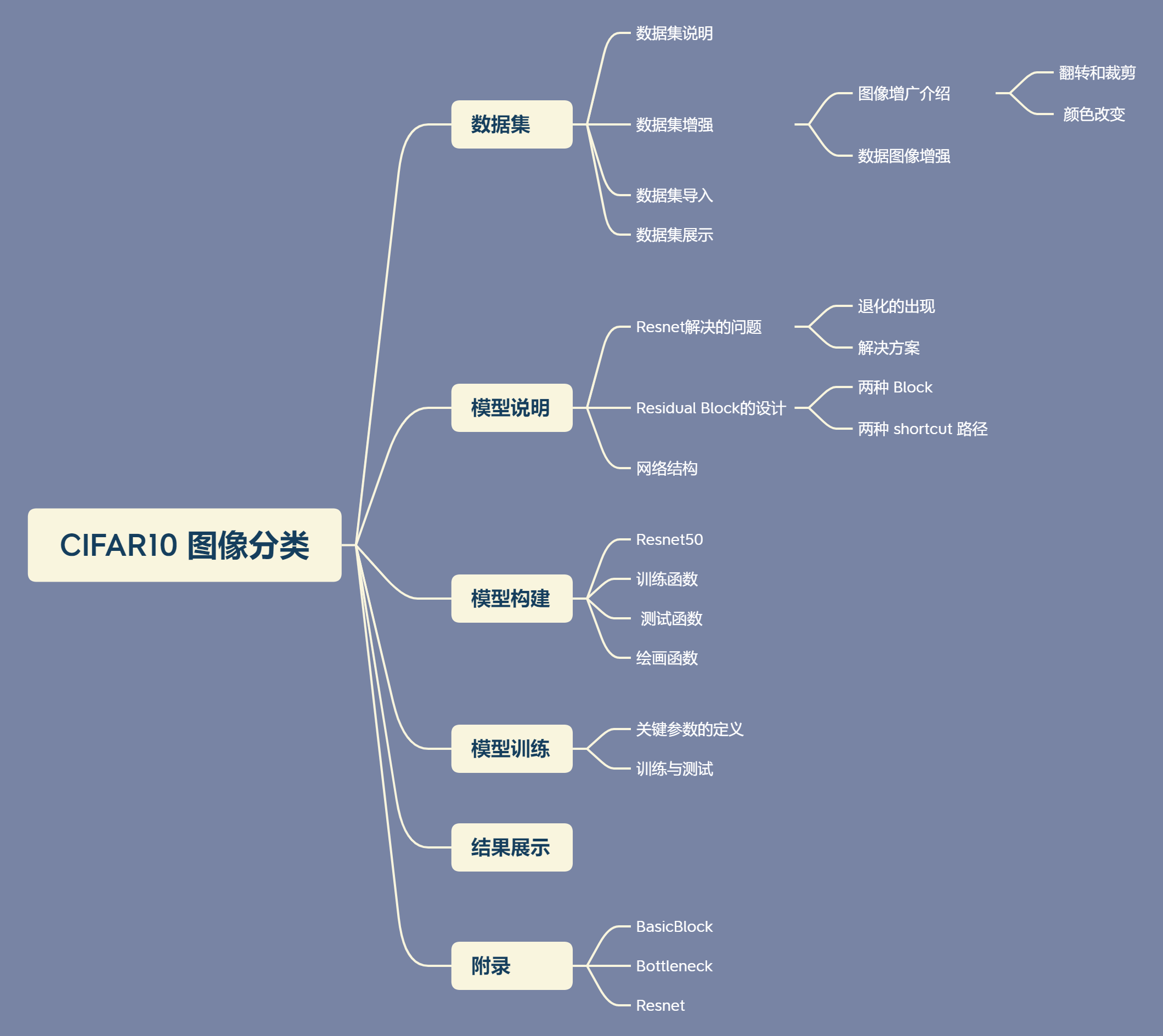

  

一、数据集

1. 数据集说明

• CIFAR-10数据集共有60000张彩色图像，这些图像是32*32，分为10个类，每类6000张图。这里面有50000张用于训练，构成了5个训练批，每一批10000张图；另外10000用于测试，单独构成一批。

编号	类别
0	airplane
1	automobile
2	brid
3	cat
4	deer
5	dog
6	frog
7	horse
8	ship
9	truck’

2. 数据集增强

1). 图像增广介绍

• 大型数据集是成功应用深度神经网络的先决条件。 图像增广在对训练图像进行一系列的随机变化之后，生成相似但不同的训练样本，从而扩大了训练集的规模。 此外，应用图像增广的原因是，随机改变训练样本可以减少模型对某些属性的依赖，从而提高模型的泛化能力。 例如，我们可以以不同的方式裁剪图像，使感兴趣的对象出现在不同的位置，减少模型对于对象出现位置的依赖

def apply(img, aug, num_rows=2, num_cols=4, scale=1.5):
    Y = [aug(img) for _ in range(num_rows * num_cols)]
    d2l.show_images(Y, num_rows, num_cols, scale=scale)

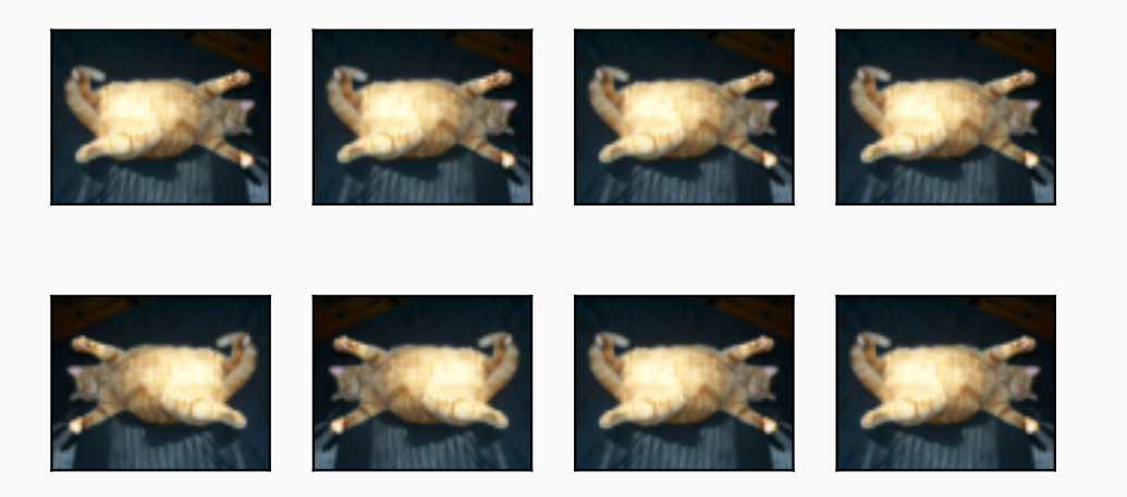
a. 翻转和裁剪

1. 翻转
   • 左右翻转图像通常不会改变对象的类别。左右翻转图像通常不会改变对象的类别。这是最早且最广泛使用的图像增广方法之一。
   • 上下翻转图像不如左右图像翻转那样常用。但是，至少对于这个示例图像，上下翻转不会妨碍识别。

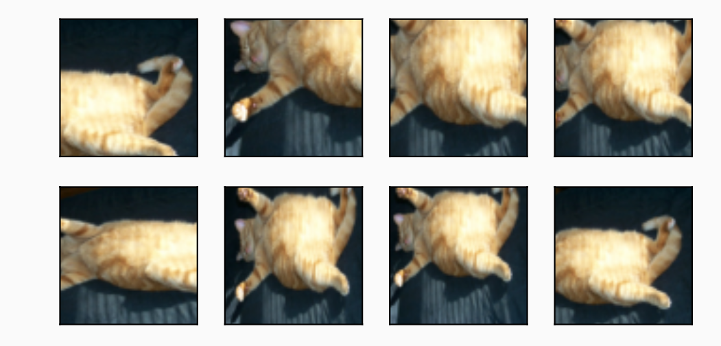
2. 裁剪
   • 可以通过对图像进行随机裁剪，使物体以不同的比例出现在图像的不同位置。 这也可以降低模型对目标位置的敏感性。（在下面的代码中，随机裁剪一个面积为原始面积10%到100%的区域，该区域的宽高比从0.5到2之间随机取值）

shape_aug = torchvision.transforms.RandomResizedCrop(
    (200, 200), scale=(0.1, 1), ratio=(0.5, 2))
apply(img, shape_aug)

b. 颜色改变

• 可以改变图像颜色的四个方面：亮度、对比度、饱和度和色调。

1. 随机更改图像的亮度

   

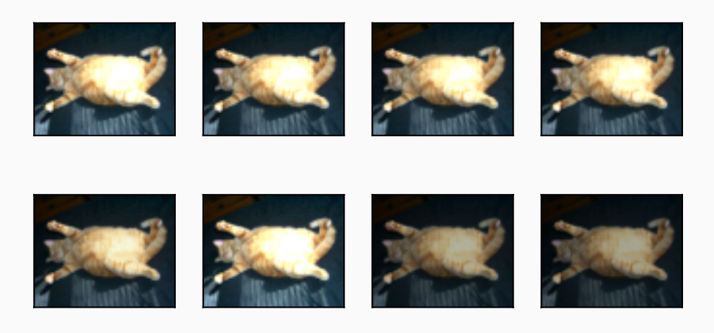
2. 可以随机更改图像的色调

   

2) 数据图像增强

stats = ((0.5,0.5,0.5),(0.5,0.5,0.5))
# 将大小转化为 -1到1
# 随即垂直 水平 翻转 默认 p=0.5

train_transform = tt.Compose([
    tt.RandomHorizontalFlip(p=0.5),
    tt.RandomVerticalFlip(p=0.5),
    tt.RandomCrop(32, padding=4, padding_mode="reflect"),
    tt.ToTensor(),
    tt.Normalize(*stats)
])

test_transform = tt.Compose([
    tt.ToTensor(),
    tt.Normalize(*stats)
])

• 对训练集 在数据集导入过程中随机上下，左右翻转（p=0.5),
• 因原数据图片不大，在经过padding = 4后对训练集进行随即裁剪
• 将训练集与测试集利用torchvision.transforms.Normalize()进行数据集归一化

3. 数据集导入

train_data = CIFAR10(download=True,root="Data", transform=train_transform)
test_data = CIFAR10(root="Data", train=False, transform=test_transform)

BATCH_SIZE = 128
train_dl = DataLoader(train_data, BATCH_SIZE, num_workers=4, pin_memory=True, shuffle=True)
test_dl = DataLoader(test_data, BATCH_SIZE, num_workers=4, pin_memory=True)

• 数据集占比例展示

  'frog': 		5000			1000
  'truck': 		5000			1000
  'deer': 		5000			1000
  'automobile': 	5000			1000
  'bird': 		5000			1000
  'horse': 		5000			1000
  'ship': 		5000			1000
  'cat': 			5000			1000
  'dog': 			5000			1000
  'airplane': 	5000			1000
  

  图像大小$32\ast 32$，分为10个类，每类6000张图。这里面有50000张用于训练，构成了训练集；另外10000张用于测试，构成测试集

4. 数据集展示

# for 8 images
train_8_samples = DataLoader(train_data, 8, num_workers=4, pin_memory=True, shuffle=True)

dataiter = iter(train_8_samples)
images, labels = dataiter.next()

fig, axs = plt.subplots(2, 4, figsize=(16, 6))
nums = 0
for i in range(2):
    for j in range(4):
        img = images[nums] / 2 + 0.5        
        npimg = img.numpy()
        axs[i][j].imshow(np.transpose(npimg, (1, 2, 0)))
        axs[i][j].set_title(train_data.classes[labels[nums]])
        nums += 1
plt.show()

二、模型说明

1.Resnet解决的问题

1.1 退化的出现

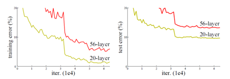
• 我们知道，对浅层网络逐渐 叠加$layers$，模型在训练集和测试集上的性能会变好，因为模型复杂度更高了，表达能力更强了，可以对潜在的映射关系拟合得更好。而**“退化”指的是，给网络叠加更多的层后，性能却快速下降的情况。**

1.2 解决方案

1. 调整求解方法，比如更好的初始化、更好的梯度下降算法等
2. 调整模型结构，让模型更易于优化——改变模型结构实际上是改变了error surface的形态

ResNet的作者从后者入手，探求更好的模型结构。将堆叠的几层$layer$称之为一个$block$，对于某个$block$，其可以拟合的函数为$F(x)$，如果期望的潜在映射为$H(x)$，与其让$F(x)$直接学习潜在的映射，不如去学习残差$H(x)-x$,即$F(x)=H(x)-x$，这样原本的前向路径上就变成了$F(x)+x$，用$F(x)+x$来拟合$H(x)$。作者认为这样可能更易于优化，因为相比于让$F(x)$学习成恒等映射，让$F(X)$学习成$0$要更加容易——后者通过$L2$正则就可以轻松实现。这样，对于冗余的block，只需$F(x)\to 0$就可以得到恒等映射，性能不减。

Instead of hoping each few stacked layers directly fit a desired underlying mapping, we explicitly let these layers fit a residual mapping. Formally, denoting the desired underlying mapping as H(x), we let the stacked nonlinear layers fit another mapping of F(x):=H(x)-x. The original mapping is recast into F(x)+x. We hypothesize that it is easier to optimize the residual mapping than to optimize the original, unreferenced mapping. To the extreme, if an identity mapping were optimal, it would be easier to push the residual to zero than to fit an identity mapping by a stack of nonlinear layers.

—— from Deep Residual Learning for Image Recognition

2. Residual Block的设计

$F(x)+x$构成的$block$称之为Residual Block，即残差块，如下图所示，多个相似的$ResidualBlock$串联构成ResNet

一个残差块有2条路径$F(x)$和$x$，$F(x)$路径拟合残差，不妨称之为残差路径，$x$路径为identity mapping恒等映射，称之为”$shortcut$”。图中的⊕为element-wise addition，要求参与运算的$F(x)$和$x$的尺寸要相同。

2.1 两种 Block

• 在原论文中，残差路径可以大致分成2种，一种有bottleneck结构，即下图右中的1×1 卷积层，用于先降维再升维，主要出于降低计算复杂度的现实考虑，称之为“bottleneck block”，另一种没有bottleneck结构，如下图左所示，称之为“basic block”。

2.2 两种 shortcut 路径

• shortcut路径大致也可以分成2种，取决于残差路径是否改变了feature map数量和尺寸，一种是将输入xx原封不动地输出，另一种则需要经过1×1卷积来升维 or/and 降采样，主要作用是将输出与F(x)路径的输出保持shape一致，对网络性能的提升并不明显，两种结构如下图所示

3. 网络结构

ResNet的设计有如下特点：

• 与plain net相比，ResNet多了很多“旁路”，即shortcut路径，其首尾圈出的layers构成一个Residual Block；

• ResNet中，所有的Residual Block都没有pooling层，降采样是通过$conv$的$stride$实现的；

• 分别在$conv{3}_1、conv{4}_1和conv{5}_{1}ResidualBlock$，降采样$1$倍，同时$featuremap$数量增加1倍，如图中虚线划定的$block$；

• 通过$AveragePooling$得到最终的特征，而不是通过全连接层；

• 每个卷积层之后都紧接着$BatchNormlayer$，为了简化，图中并没有标出；

三、模型构建

1. Resnet50

class Bottleneck(nn.Module):
    expansion = 4

    def __init__(self, in_planes, planes, stride=1):
        super(Bottleneck, self).__init__()
        self.conv1 = nn.Conv2d(in_planes, planes, kernel_size=1, bias=False)
        self.bn1 = nn.BatchNorm2d(planes)
        self.conv2 = nn.Conv2d(planes, planes, kernel_size=3,
                               stride=stride, padding=1, bias=False)
        self.bn2 = nn.BatchNorm2d(planes)
        self.conv3 = nn.Conv2d(planes, self.expansion *
                               planes, kernel_size=1, bias=False)
        self.bn3 = nn.BatchNorm2d(self.expansion*planes)

        self.shortcut = nn.Sequential()
        if stride != 1 or in_planes != self.expansion*planes:
            self.shortcut = nn.Sequential(
                nn.Conv2d(in_planes, self.expansion*planes,
                          kernel_size=1, stride=stride, bias=False),
                nn.BatchNorm2d(self.expansion*planes)
            )

    def forward(self, x):
        out = F.relu(self.bn1(self.conv1(x)))
        out = F.relu(self.bn2(self.conv2(out)))
        out = self.bn3(self.conv3(out))
        out += self.shortcut(x)
        out = F.relu(out)
        return out

class ResNet(nn.Module):
    def __init__(self, block, num_blocks, num_classes=10):
        super(ResNet, self).__init__()
        self.in_planes = 64

        self.conv1 = nn.Conv2d(3, 64, kernel_size=3,
                               stride=1, padding=1, bias=False)
        self.bn1 = nn.BatchNorm2d(64)
        self.layer1 = self._make_layer(block, 64, num_blocks[0], stride=1)
        self.layer2 = self._make_layer(block, 128, num_blocks[1], stride=2)
        self.layer3 = self._make_layer(block, 256, num_blocks[2], stride=2)
        self.layer4 = self._make_layer(block, 512, num_blocks[3], stride=2)
        self.linear = nn.Linear(512*block.expansion, num_classes)

    def _make_layer(self, block, planes, num_blocks, stride):
        strides = [stride] + [1]*(num_blocks-1)
        layers = []
        for stride in strides:
            layers.append(block(self.in_planes, planes, stride))
            self.in_planes = planes * block.expansion
        return nn.Sequential(*layers)

    def forward(self, x):
        out = F.relu(self.bn1(self.conv1(x)))
        out = self.layer1(out)
        out = self.layer2(out)
        out = self.layer3(out)
        out = self.layer4(out)
        out = F.avg_pool2d(out, 4)
        out = out.view(out.size(0), -1)
        out = self.linear(out)
        return out
    
def ResNet50():
    return ResNet(Bottleneck, [3, 4, 6, 3])

2. 训练函数

def train(epoch):
    net.train()
    epoch_loss = 0
    correct = 0
    total = 0
    for batch_idx, (inputs, targets) in enumerate(train_dl):
        inputs, targets = inputs.to(device), targets.to(device)
        optimizer.zero_grad()
        outputs = net(inputs)
        loss = criterion(outputs, targets)
        loss.backward()
        optimizer.step()

        epoch_loss += loss.item()* inputs.size(0)
        _, predicted = outputs.max(1)
        total += targets.size(0)
        correct += predicted.eq(targets).sum().item()
    acc = correct / total
    loss = epo

3. 测试函数

def test(epoch):
    global best_acc
    net.eval()
    epoch_loss = 0
    correct = 0
    total = 0
    with torch.no_grad():
        for batch_idx, (inputs, targets) in enumerate(test_dl):
            inputs, targets = inputs.to(device), targets.to(device)
            outputs = net(inputs)
            loss = criterion(outputs, targets)

            epoch_loss += loss.item()* inputs.size(0)
            _, predicted = outputs.max(1)
            total += targets.size(0)
            correct += predicted.eq(targets).sum().item()
    acc = correct / total
    loss = epoch_loss / total

    print('test_loss: %.4f test_acc: %.4f '%(loss, acc), end=' ' )
    return {'loss': loss, 'acc': acc}

4. 绘画函数

def plot(d, mode='train', best_acc_=None):
    import matplotlib.pyplot as plt
    plt.figure(figsize=(10, 4))
    plt.suptitle('%s_curve' % mode)
    plt.subplots_adjust(wspace=0.2, hspace=0.2)
    epochs = len(d['acc'])

    plt.subplot(1, 2, 1)
    plt.plot(np.arange(epochs), d['loss'], label='loss')
    plt.xlabel('epoch')
    plt.ylabel('loss')
    plt.legend(loc='upper left')

    plt.subplot(1, 2, 2)
    plt.plot(np.arange(epochs), d['acc'], label='acc')
    if best_acc_ is not None:
        plt.scatter(best_acc_[0], best_acc_[1], c='r')
    plt.xlabel('epoch')
    plt.ylabel('acc')
    plt.legend(loc='upper left')
    plt.savefig('resnet50_cifar10_%s.jpg' % mode, bbox_inches='tight')

四、模型训练

1. 关键参数的定义

parser = argparse.ArgumentParser(description='PyTorch CIFAR10 Training')
parser.add_argument('--lr', default=0.1, type=float, help='learning rate')
args = parser.parse_args(args=[])
device = 'cuda' if torch.cuda.is_available() else 'cpu'

net = ResNet50()
net = net.to(device)

criterion = nn.CrossEntropyLoss()
optimizer = optim.SGD(net.parameters(), lr=args.lr,
                      momentum=0.9, weight_decay=5e-4)
scheduler = torch.optim.lr_scheduler.CosineAnnealingLR(optimizer, T_max=60)

2. 训练与测试

train_info = {'loss': [], 'acc': []}
test_info = {'loss': [], 'acc': []}
for epoch in range(61):
    time1 = time.time()
    d_train = train(epoch)
    d_test = test(epoch)
    scheduler.step()
    print("%.4ss"%(time.time() - time1), end='\n')
    for k in train_info.keys():
        train_info[k].append(d_train[k])
        test_info[k].append(d_test[k])

五、 结果展示

• 展示后10个epoch的过程

  epoches: 50 train_loss: 0.1613 train_acc: 0.9437  --> test_loss: 0.3568 test_acc: 0.8886  73.6s
  epoches: 51 train_loss: 0.1445 train_acc: 0.9496  --> test_loss: 0.3252 test_acc: 0.8972  73.6s
  epoches: 52 train_loss: 0.1303 train_acc: 0.9549  --> test_loss: 0.3224 test_acc: 0.9002  73.5s
  epoches: 53 train_loss: 0.1125 train_acc: 0.9614  --> test_loss: 0.3165 test_acc: 0.9013  73.5s
  epoches: 54 train_loss: 0.0976 train_acc: 0.9667  --> test_loss: 0.3100 test_acc: 0.9073  73.5s
  epoches: 55 train_loss: 0.0871 train_acc: 0.9709  --> test_loss: 0.3152 test_acc: 0.9072  73.5s
  epoches: 56 train_loss: 0.0795 train_acc: 0.9733  --> test_loss: 0.3089 test_acc: 0.9092  73.5s
  epoches: 57 train_loss: 0.0731 train_acc: 0.9754  --> test_loss: 0.3033 test_acc: 0.9114  73.5s
  epoches: 58 train_loss: 0.0719 train_acc: 0.9759  --> test_loss: 0.3004 test_acc: 0.9106  73.5s
  epoches: 59 train_loss: 0.0679 train_acc: 0.9784  --> test_loss: 0.3028 test_acc: 0.9111  73.5s
  epoches: 60 train_loss: 0.0678 train_acc: 0.9781  --> test_loss: 0.3027 test_acc: 0.9113  73.5s
  

• 在本次训练中 测试集最优 acc 达到了91.14% 较好的完成了预期

附录

基于PyTorch的Resnet实现

1. BasicBlock

import torch
import torch.nn as nn
import torch.nn.functional as F

class BasicBlock(nn.Module):
   
`	expansion = 1

    def __init__(self, in_planes, planes, stride=1):
        super(BasicBlock, self).__init__()
        self.conv1 = nn.Conv2d(
            in_planes, planes, kernel_size=3, stride=stride, padding=1, bias=False)
        self.bn1 = nn.BatchNorm2d(planes)
        self.conv2 = nn.Conv2d(planes, planes, kernel_size=3,
                               stride=1, padding=1, bias=False)
        self.bn2 = nn.BatchNorm2d(planes)

        self.shortcut = nn.Sequential()
        if stride != 1 or in_planes != self.expansion*planes:
            self.shortcut = nn.Sequential(
                nn.Conv2d(in_planes, self.expansion*planes,
                          kernel_size=1, stride=stride, bias=False),
                nn.BatchNorm2d(self.expansion*planes)
            )

    def forward(self, x):
        out = F.relu(self.bn1(self.conv1(x)))
        out = self.bn2(self.conv2(out))
        out += self.shortcut(x)
        out = F.relu(out)
        return out

2. Bottleneck

class Bottleneck(nn.Module):
    
    expansion = 4

    def __init__(self, in_planes, planes, stride=1):
        super(Bottleneck, self).__init__()
        self.conv1 = nn.Conv2d(in_planes, planes, kernel_size=1, bias=False)
        self.bn1 = nn.BatchNorm2d(planes)
        self.conv2 = nn.Conv2d(planes, planes, kernel_size=3,
                               stride=stride, padding=1, bias=False)
        self.bn2 = nn.BatchNorm2d(planes)
        self.conv3 = nn.Conv2d(planes, self.expansion *
                               planes, kernel_size=1, bias=False)
        self.bn3 = nn.BatchNorm2d(self.expansion*planes)

        self.shortcut = nn.Sequential()
        if stride != 1 or in_planes != self.expansion*planes:
            self.shortcut = nn.Sequential(
                nn.Conv2d(in_planes, self.expansion*planes,
                          kernel_size=1, stride=stride, bias=False),
                nn.BatchNorm2d(self.expansion*planes)
            )

    def forward(self, x):
        out = F.relu(self.bn1(self.conv1(x)))
        out = F.relu(self.bn2(self.conv2(out)))
        out = self.bn3(self.conv3(out))
        out += self.shortcut(x)
        out = F.relu(out)
        return out

3. Resnet

class ResNet(nn.Module):
    def __init__(self, block, num_blocks, num_classes=10):
        super(ResNet, self).__init__()
        self.in_planes = 64

        self.conv1 = nn.Conv2d(3, 64, kernel_size=3,
                               stride=1, padding=1, bias=False)
        self.bn1 = nn.BatchNorm2d(64)
        self.layer1 = self._make_layer(block, 64, num_blocks[0], stride=1)
        self.layer2 = self._make_layer(block, 128, num_blocks[1], stride=2)
        self.layer3 = self._make_layer(block, 256, num_blocks[2], stride=2)
        self.layer4 = self._make_layer(block, 512, num_blocks[3], stride=2)
        self.linear = nn.Linear(512*block.expansion, num_classes)

    def _make_layer(self, block, planes, num_blocks, stride):
        strides = [stride] + [1]*(num_blocks-1)
        layers = []
        for stride in strides:
            layers.append(block(self.in_planes, planes, stride))
            self.in_planes = planes * block.expansion
        return nn.Sequential(*layers)

    def forward(self, x):
        out = F.relu(self.bn1(self.conv1(x)))
        out = self.layer1(out)
        out = self.layer2(out)
        out = self.layer3(out)
        out = self.layer4(out)
        out = F.avg_pool2d(out, 4)
        out = out.view(out.size(0), -1)
        out = self.linear(out)
        return out

# 默认 num_classes=10
def ResNet18():
    return ResNet(BasicBlock, [2, 2, 2, 2])
    
def ResNet34():
    return ResNet(BasicBlock, [3, 4, 6, 3])

def ResNet50():
    return ResNet(Bottleneck, [3, 4, 6, 3])

def ResNet101():
    return ResNet(Bottleneck, [3, 4, 23, 3])

def ResNet152():
    return ResNet(Bottleneck, [3, 8, 36, 3])

参考链接：动手学深度学习