python scipy.optimize 求解带边界约束的非线性规划报错“Positive directional derivative for linesearch”

问题背景

在数据处理过程中，需要求解形如下图的非线性规划：
　　
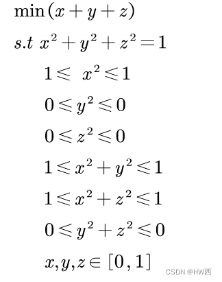
　　（在我的学习任务中不等式约束边界会变化，上图示意一个特殊情况）

求解方法一：scipy.optimize

尝试利用scipy.optimize中的．minimize（）函数进行求解，将等式与不等式约束存入cons字典中。

from scipy.optimize import minimize
import numpy as np

fun = lambda x :　x[0] + x[1] + x[2]# 约束函数
cons = ({'type': 'eq', 'fun': lambda x: x[0]**2+ x[1]**2+ x[2]**2 - 1}, # xyz=1

{'type': 'ineq', 'fun': lambda x: 1-x[0]**2 },#  1 >= x**2
{'type': 'ineq', 'fun': lambda x: x[0]**2-1 },#  x**2 >=1

{'type': 'ineq', 'fun': lambda x: 0-x[1]**2 },
{'type': 'ineq', 'fun': lambda x: x[1]**2- 0 },

{'type': 'ineq', 'fun': lambda x:  0-x[2]**2 },
{'type': 'ineq', 'fun': lambda x: x[2]**2-0 },

{'type': 'ineq', 'fun': lambda x: 1-x[0]**2-x[1]**2 },
{'type': 'ineq', 'fun': lambda x: x[0]**2+x[1]**2 -1},

{'type': 'ineq', 'fun': lambda x: 1-x[0]**2-x[2]**2 },
{'type': 'ineq', 'fun': lambda x: x[0]**2+x[2]**2-1}，

{'type': 'ineq', 'fun': lambda x: 0-x[1]**2-x[2]**2 },
{'type': 'ineq', 'fun': lambda x: x[1]**2+x[2]**2- 0 }
)
b1=(0,1)
b2=(0,1)
b3=(0,1)
bonds=(b1,b2,b3)
x0 = np.array((0.5, 0.5, 0.5)) # 设置初始值
res = minimize(fun, x0, method='SLSQP', constraints=cons,bounds=bonds, 
              tol=None)
#print(np.around(res.x,4))#量子形式的系数
print('最小值：',res.fun)
print('最优解：',res.x)
print('迭代终止是否成功：', res.success)
print('迭代终止原因：', res.message)

运行结果：

问题：

1. 明显该规划问题的最优解为(1, 0, 0)，但运行结果计算错误。通过查看具体运行信息，可以发现迭代终止并未成功，并给出了‘Positive directional derivative for linesearch’信息；
2. 该规划需要对初始值进行声明，即x0 = np.array((0.5, 0.5, 0.5))部分，且初始值的设定对运行结果影响很大，若设x0 = np.array((1, 0, 0))，则运行可以成功，明显不符合一般计算逻辑。

其他：
　　尝试过一些其他解决方法，指路Positive directional derivative for linesearch的四种解决方案，Python 的 scipy.optimize.minimize 与 SLSQP 失败并显示 “Positive directional derivative for linesearch”，均无法成功运行。最终尝试替换计算方法，使用差分进化算法进行求解（指路差分进化算法解决有约束优化问题（Python）），具体过程如下：

求解方法二：差分进化算法

from sko.DE import DE

def obj_func(p):
    x1, x2, x3 = p
    return x1 + x2  + x3 

constraint_eq = [lambda x: 1 -x[0]**2 - x[1]**2 - x[2]**2]

constraint_ueq = [lambda x: 1-x[0]**2, lambda x: x[0]**2-1,
                  lambda x: 0-x[1]**2,lambda x: x[1]**2- 0,
                  lambda x: 0-x[2]**2,lambda x: x[2]**2- 0,
                  lambda x: 1-x[0]**2-x[1]**2,lambda x: x[0]**2+x[1]**2 -1,
                  lambda x: 1-x[0]**2-x[2]**2,lambda x: x[0]**2+x[2]**2-1,
                  lambda x: 0-x[1]**2-x[2]**2,lambda x: x[1]**2+x[2]**2- 0                
                 ]
de = DE(func=obj_func, n_dim=3, size_pop=50, max_iter=100, lb=[0, 0, 0], ub=[1, 1, 1],
        constraint_eq=constraint_eq, constraint_ueq=constraint_ueq)
best_x, best_y = de.run()

print('best_x:', np.around(best_x,2), '\n', 'best_y:', best_y)

运行结果：

总结：

从计算结果来看，差分进化算法不但不需要指定初始值，也可以成功计算一些特殊情况，此外针对更一般的边界约束情况，上述规划仍可成功计算。因此方法二更适用于本问题。