2021-11-04 统计学-基于R（第四版）第六章课后习题记录及总结

先声明，本博客为我的个人作业，不保证一定为标准答案！

6.1 题目如下

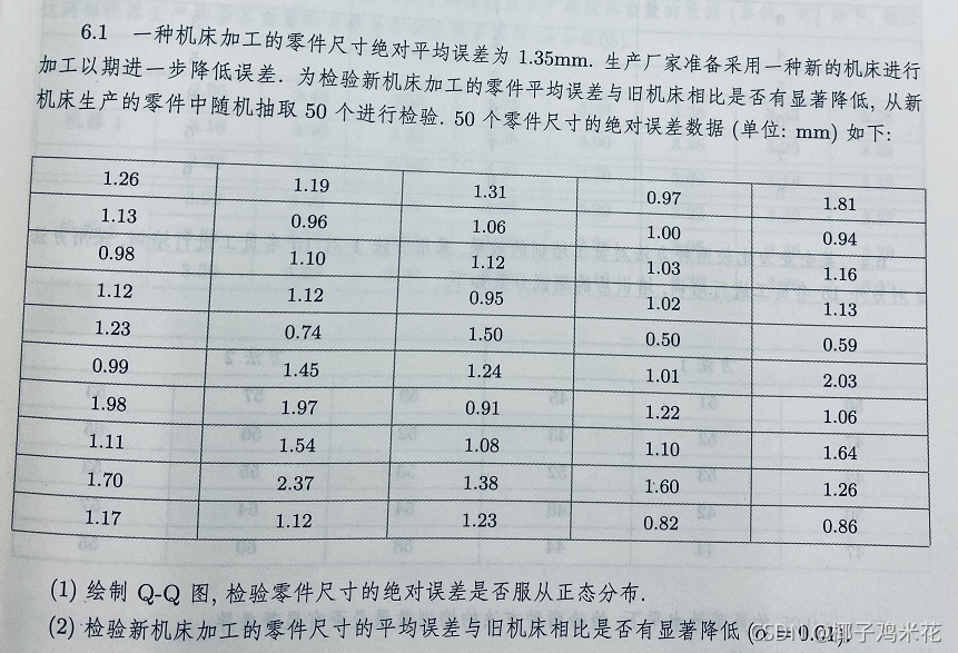
 （1）代码如下：

> example6_1<-read.csv("D:/作业/统计学R/《统计学—基于R》（第4版）—例题和习题数据（公开资源）/exercise/chap06/exercise6_1.csv")
> par(mai=c(0.6,0.6,0.2,0.2),cex=0.7,mgp=c(2,1,0))
> qqnorm(example6_1$零件误差,xlab="期望正态值",ylab="观测值")
> qqline(example6_1$零件误差,col="red",lwd=2)

画出来的Q-Q图为

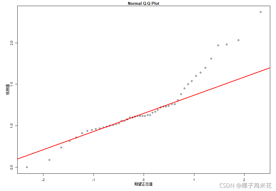
 Q-Q图显示零件尺寸的绝对误差不服从正态分布

（2）

H₀:μ>=1.35  H₁:μ<1.35

> library(BSDA)
> z.test(example6_1$零件误差,mu=1.35,sigma.x=sd(example6_1$零件误差),alternative="less",conf.level=0.99)

	One-sample z-Test

data:  example6_1$零件误差
z = -2.6061, p-value = 0.004579
alternative hypothesis: true mean is less than 1.35
99 percent confidence interval:
      NA 1.33553
sample estimates:
mean of x 
   1.2152 

p-value = 0.004579<0.01，拒绝原假设，新机床加工的零件尺寸的平均误差与旧机床相比显著降低

---

6.2 题目如下

 

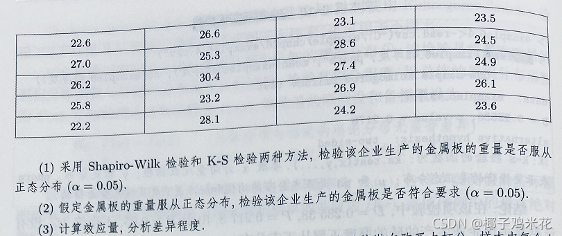
 （1）Shapiro-Wilk检验：

> example6_2<-read.csv("D:/作业/统计学R/《统计学—基于R》（第4版）—例题和习题数据（公开资源）/exercise/chap06/exercise6_2.csv")
> shapiro.test(example6_2$重量)

	Shapiro-Wilk normality test

data:  example6_2$重量
W = 0.97064, p-value = 0.7684

K-S检验：

> ks.test(example6_2$重量,"pnorm",mean(example6_2$重量),sd(example6_2$重量))

	One-sample Kolmogorov-Smirnov
	test

data:  example6_2$重量
D = 0.10808, p-value = 0.9539
alternative hypothesis: two-sided

检验的p值均大于0.05，不拒绝原假设，可以认为该企业生产的金属板的重量服从正态分布

（2）

H₀:μ=25  H₁:μ！=25

> t.test(example6_2$重量,mu=25,conf.level=0.95)

	One Sample t-test

data:  example6_2$重量
t = 1.0399, df = 19, p-value =
0.3114
alternative hypothesis: true mean is not equal to 25
95 percent confidence interval:
 24.48352 26.53648
sample estimates:
mean of x 
    25.51 

p-value =0.3114>0.05，不拒绝原假设，可以认为该企业生产的金属板的重量符合要求

（3）

> library(lsr)
> cohensD(example6_2$重量,mu=25)
[1]0.2325298

该企业生产的金属板的平均重量与标准重量相差0.2325298个标准差

---

6.3 题目如下

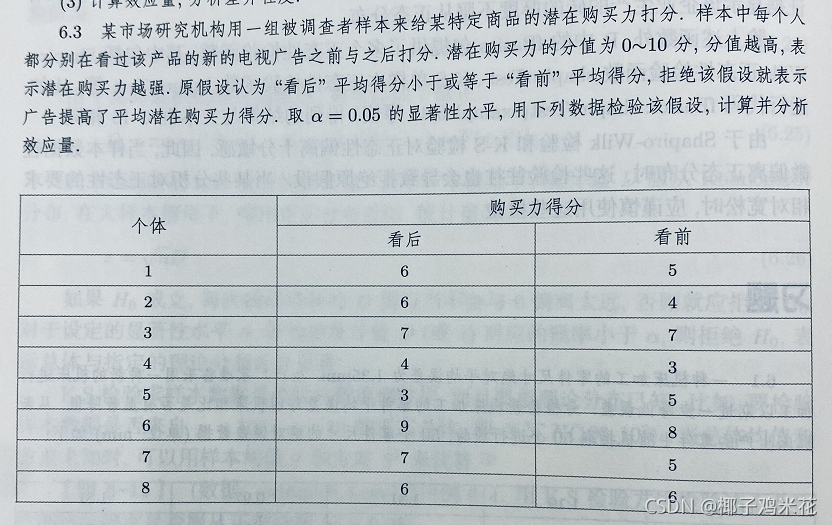
看后得分μ₁，看前得分μ₂

H₀:μ₁-μ₂<=0  H₁:μ₁-μ₂>0

> example6_3<-read.csv("D:/作业/统计学R/《统计学—基于R》（第4版）—例题和习题数据（公开资源）/exercise/chap06/exercise6_3.csv")
> t.test(example6_3$看后,example6_3$看前,alternative="greater",paired=TRUE)

	Paired t-test

data:  example6_3$看后 and example6_3$看前
t = 1.3572, df = 7, p-value =
0.1084
alternative hypothesis: true difference in means is greater than 0
95 percent confidence interval:
 -0.2474397        Inf
sample estimates:
mean of the differences 
                  0.625 

p-value =0.1084>0.05，不拒绝原假设，广告没有提高平均潜在购买力得分

> library(lsr)
> cohensD(example6_3$看后,example6_3$看前,method="paired")
[1]0.4798574

效应量为0.4798574，该检验结果属于小的效应量

---

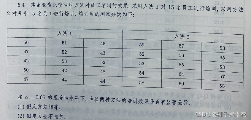
6.4 题目如下

 

方法1平均分数μ₁，方法2平均分数μ₂

H₀:μ₁-μ₂=0  H₁:μ₁-μ₂！=0

（1）

> example6_4<-read.csv("D:/作业/统计学R/《统计学—基于R》（第4版）—例题和习题数据（公开资源）/exercise/chap06/exercise6_4.csv")
> t.test(example6_4$方法1,example6_4$方法2,var.equal=TRUE)

	Two Sample t-test

data:  example6_4$方法1 and example6_4$方法2
t = -5.8927, df = 28, p-value =
2.444e-06
alternative hypothesis: true difference in means is not equal to 0
95 percent confidence interval:
 -12.128568  -5.871432
sample estimates:
mean of x mean of y 
 47.73333  56.73333 

p-value =2.444e-06<0.05，拒绝原假设，两种方法的培训效果有显著差异

（2）

> t.test(example6_4$方法1,example6_4$方法2,var.equal=FALSE)

	Welch Two Sample t-test

data:  example6_4$方法1 and example6_4$方法2
t = -5.8927, df = 27.639,
p-value = 2.568e-06
alternative hypothesis: true difference in means is not equal to 0
95 percent confidence interval:
 -12.130411  -5.869589
sample estimates:
mean of x mean of y 
 47.73333  56.73333 

p-value =2.568e-06<0.05，拒绝原假设，两种方法的培训效果有显著差异

（3）

> library(lsr)
> cohensD(example6_4$方法1,example6_4$方法2)
[1]2.151704

效应量为2.151704，该检验结果属于大的效应量

---

6.5 题目如下

 H₀:π<=17%  H₁:π>17%

> n<-550
> p<-115/550
> piO<-0.17
> z<-(p-piO)/sqrt(piO*(1-piO)/n)
> p_value<-1-pnorm(z)
> data.frame(z,p_value)
         z     p_value
1 2.440583 0.007331785

p_value=0.007331785<0.05，拒绝原假设，该生产商的说法属实

---

6.6 题目如下

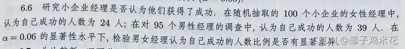
女经理平均成功比例π₁，男经理平均成功比例π₂

H₀:π₁-π₂=0  H₁:π₁-π₂！=0

> n1<-100
> n2<-95
> p1<-24/100
> p2<-39/95
> p<-(p1*n1+p2*n2)/(n1+n2)
> z<-(p1-p2)/sqrt(p*(1-p)*(1/n1+1/n2))
> p_value<-pnorm(z)
> data.frame(z,p_value)
          z    p_value
1 -2.545149 0.00546155

p_value=0.00546155<0.06，拒绝原假设，男女经理认为自己成功的人数比例有显著差异

---

6.7 题目如下 

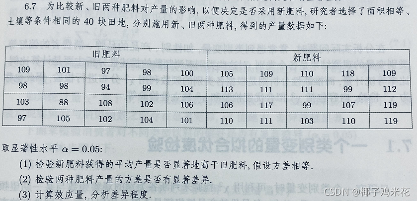
（1）

新肥料产量均值μ₁，旧肥料产量均值μ₂

H₀:μ₁-μ₂<=0  H₁:μ₁-μ₂>0

> example6_7<-read.csv("D:/作业/统计学R/《统计学—基于R》（第4版）—例题和习题数据（公开资源）/exercise/chap06/exercise6_7.csv")
> t.test(example6_7$新肥料,example6_7$旧肥料,var.qual=TRUE)

	Welch Two Sample t-test

data:  example6_7$新肥料 and example6_7$旧肥料
t = 5.4271, df = 37.042,
p-value = 3.735e-06
alternative hypothesis: true difference in means is not equal to 0
95 percent confidence interval:
  5.765342 12.634658
sample estimates:
mean of x mean of y 
    109.9     100.7 

p-value = 3.735e-06<0.05，拒绝原假设，新肥料获得的平均产量显著高于旧肥料

（2）

新肥料产量方差σ₁²，旧肥料产量方差σ₂²

H₀:σ₁²/σ₂²=1  H₁:σ₁²/σ₂²!=1

> var.test(example6_7$新肥料,example6_7$旧肥料,alternative="two.sided")

	F test to compare two
	variances

data:  example6_7$新肥料 and example6_7$旧肥料
F = 1.3832, num df = 19, denom
df = 19, p-value = 0.4862
alternative hypothesis: true ratio of variances is not equal to 1
95 percent confidence interval:
 0.5475027 3.4946849
sample estimates:
ratio of variances 
          1.383239 

p-value = 0.4862>0.05，不拒绝原假设，两种肥料产量的方差无显著差异

（3）

> library(lsr)
> cohensD(example6_7$新肥料,example6_7$旧肥料)
[1]1.716202

效应量为1.716202，为大的效应量

---

6.8 题目如下 

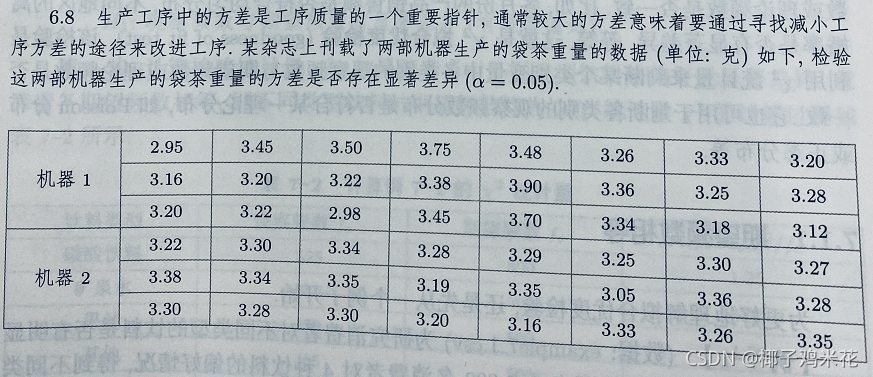
机器1生产的袋茶重量方差σ₁²，机器2生产的袋茶重量方差σ₂²

H₀:σ₁²/σ₂²=1  H₁:σ₁²/σ₂²!=1

> example6_8<-read.csv("D:/作业/统计学R/《统计学—基于R》（第4版）—例题和习题数据（公开资源）/exercise/chap06/exercise6_8.csv")
> var.test(example6_8$机器1,example6_8$机器2,alternative="two.sided")

	F test to compare two
	variances

data:  example6_8$机器1 and example6_8$机器2
F = 9.0711, num df = 23, denom
df = 23, p-value = 1.477e-06
alternative hypothesis: true ratio of variances is not equal to 1
95 percent confidence interval:
  3.924078 20.969026
sample estimates:
ratio of variances 
          9.071058 

p-value = 1.477e-06<0.05，拒绝原假设，这两部机器生产的袋茶重量的方差无显著差异

---

本次记录就到这！