2021-12-16 统计学-基于R（第四版）第十章课后习题记录及总结

最新推荐文章于 2022-04-07 22:26:32 发布

椰子鸡米花

最新推荐文章于 2022-04-07 22:26:32 发布

阅读量4.5k

点赞数 10

分类专栏： R语言学习文章标签： r语言统计学

本文链接：https://blog.csdn.net/m0_52461904/article/details/121977742

版权

R语言学习专栏收录该内容

14 篇文章 129 订阅

订阅专栏

先声明，本博客为个人作业不一定为标准答案，仅供参考

10.1 题目如下

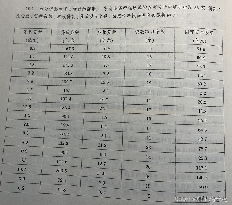
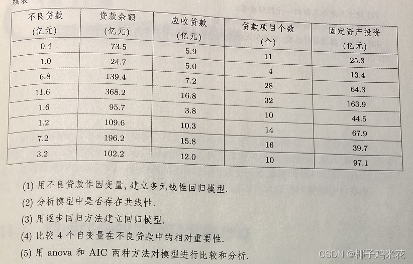
（1）

> example10_1<-read.csv("D:/作业/统计学R/《统计学—基于R》（第4版）—例题和习题数据（公开资源）/exercise/chap10/exercise10_1.csv")
> model1<-lm(不良贷款~贷款余额+应收贷款+贷款项目个数+固定资产投资,data=example10_1)
> summary(model1)

Call:
lm(formula = 不良贷款 ~ 贷款余额 + 应收贷款 + 贷款项目个数 + 
    固定资产投资, data = example10_1)

Residuals:
    Min      1Q  Median      3Q     Max 
-2.9198 -0.9507 -0.2880  1.0334  3.1037 

Coefficients:
             Estimate Std. Error t value Pr(>|t|)   
(Intercept)  -1.02164    0.78237  -1.306  0.20643   
贷款余额      0.04004    0.01043   3.837  0.00103 **
应收贷款      0.14803    0.07879   1.879  0.07494 . 
贷款项目个数  0.01453    0.08303   0.175  0.86285   
固定资产投资 -0.02919    0.01507  -1.937  0.06703 . 
---
Signif. codes:  0 ‘***’ 0.001 ‘**’ 0.01 ‘*’ 0.05 ‘.’ 0.1 ‘ ’ 1

Residual standard error: 1.779 on 20 degrees of freedom
Multiple R-squared:  0.7976,	Adjusted R-squared:  0.7571 
F-statistic:  19.7 on 4 and 20 DF,  p-value: 1.035e-06

（2）

> library(car)
> vif(model1)
    贷款余额     应收贷款 贷款项目个数 固定资产投资 
    5.330807     1.889860     3.834823     2.781220

VIF最大值为5.330807<10，显示模型的共线性在可容忍范围内

（3）

> model2<-step(model1)
Start:  AIC=33.22
不良贷款 ~ 贷款余额 + 应收贷款 + 贷款项目个数 + 固定资产投资

               Df Sum of Sq     RSS    AIC
- 贷款项目个数  1     0.097  63.376 31.255
<none>                       63.279 33.217
- 应收贷款      1    11.168  74.447 35.280
- 固定资产投资  1    11.868  75.147 35.514
- 贷款余额      1    46.594 109.873 45.011

Step:  AIC=31.26
不良贷款 ~ 贷款余额 + 应收贷款 + 固定资产投资

               Df Sum of Sq     RSS    AIC
<none>                       63.376 31.255
- 应收贷款      1    11.333  74.709 33.368
- 固定资产投资  1    12.147  75.523 33.639
- 贷款余额      1    69.939 133.315 47.846

逐步回归显示，应剔除贷款项目个数这个自变量来建立模型

逐步回归建模结果如下：

> summary(model2)

Call:
lm(formula = 不良贷款 ~ 贷款余额 + 应收贷款 + 固定资产投资, data = example10_1)

Residuals:
    Min      1Q  Median      3Q     Max 
-2.8531 -0.8766 -0.3685  0.9586  3.0772 

Coefficients:
              Estimate Std. Error t value Pr(>|t|)    
(Intercept)  -0.971605   0.711240  -1.366   0.1864    
贷款余额      0.041039   0.008525   4.814 9.31e-05 ***
应收贷款      0.148858   0.076817   1.938   0.0662 .  
固定资产投资 -0.028502   0.014206  -2.006   0.0579 .  
---
Signif. codes:  0 ‘***’ 0.001 ‘**’ 0.01 ‘*’ 0.05 ‘.’ 0.1 ‘ ’ 1

Residual standard error: 1.737 on 21 degrees of freedom
Multiple R-squared:  0.7973,	Adjusted R-squared:  0.7683 
F-statistic: 27.53 on 3 and 21 DF,  p-value: 1.802e-07

（4）

> library(lm.beta)
> model1.beta<-lm.beta(model1)
> summary(model1.beta)

Call:
lm(formula = 不良贷款 ~ 贷款余额 + 应收贷款 + 贷款项目个数 + 
    固定资产投资, data = example10_1)

Residuals:
    Min      1Q  Median      3Q     Max 
-2.9198 -0.9507 -0.2880  1.0334  3.1037 

Coefficients:
             Estimate Standardized Std. Error t value Pr(>|t|)   
(Intercept)  -1.02164      0.00000    0.78237  -1.306  0.20643   
贷款余额      0.04004      0.89131    0.01043   3.837  0.00103 **
应收贷款      0.14803      0.25982    0.07879   1.879  0.07494 . 
贷款项目个数  0.01453      0.03447    0.08303   0.175  0.86285   
固定资产投资 -0.02919     -0.32492    0.01507  -1.937  0.06703 . 
---
Signif. codes:  0 ‘***’ 0.001 ‘**’ 0.01 ‘*’ 0.05 ‘.’ 0.1 ‘ ’ 1

Residual standard error: 1.779 on 20 degrees of freedom
Multiple R-squared:  0.7976,	Adjusted R-squared:  0.7571 
F-statistic:  19.7 on 4 and 20 DF,  p-value: 1.035e-06

由标准化回归系数可知各个自变量的相对重要性依次为：贷款余额>固定资产投资>应收贷款>贷款项目个数

（5）

Anova方法：

> anova(model2,model1)
Analysis of Variance Table

Model 1: 不良贷款 ~ 贷款余额 + 应收贷款 + 固定资产投资
Model 2: 不良贷款 ~ 贷款余额 + 应收贷款 + 贷款项目个数 + 固定资产投资
  Res.Df    RSS Df Sum of Sq      F Pr(>F)
1     21 63.376                           
2     20 63.279  1  0.096877 0.0306 0.8629

p=0.8629>0.05，不拒绝H0，两个模型没有显著差异，从回归模型的简约原则看，选择逐步回归保留的3个自变量建立模型比较合适

AIC方法：

> AIC(model2,model1)
       df      AIC
model2  5 104.2022
model1  6 106.1639

AIC值越小模型越好，因此选择逐步回归模型的结果更好

10.2 题目如下

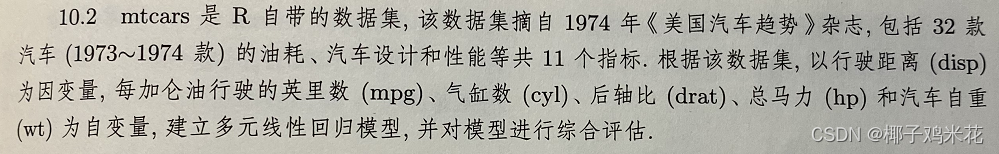
多元线性回归模型结果如下：

> model1<-lm(disp~mpg+cyl+drat+hp+wt,data=mtcars)
> summary(model1)

Call:
lm(formula = disp ~ mpg + cyl + drat + hp + wt, data = mtcars)

Residuals:
    Min      1Q  Median      3Q     Max 
-72.393 -26.432   4.697  30.160  59.418 

Coefficients:
             Estimate Std. Error t value Pr(>|t|)    
(Intercept) -233.6420   160.8590  -1.452 0.158335    
mpg            3.2249     3.1044   1.039 0.308454    
cyl           30.3927    10.5133   2.891 0.007658 ** 
drat         -13.5209    22.5147  -0.601 0.553348    
hp             0.3208     0.2187   1.467 0.154479    
wt            66.2331    16.1055   4.112 0.000348 ***
---
Signif. codes:  0 ‘***’ 0.001 ‘**’ 0.01 ‘*’ 0.05 ‘.’ 0.1 ‘ ’ 1

Residual standard error: 40.99 on 26 degrees of freedom
Multiple R-squared:  0.9082,	Adjusted R-squared:  0.8906 
F-statistic: 51.47 on 5 and 26 DF,  p-value: 1.157e-12

回归结果显示，5个自变量中，只有cyl和wt显著，其余均不显著，模型可能存在多重共线性

VIF结果如下：

> library(car)
> vif(model1)
     mpg      cyl     drat       hp       wt 
6.457610 6.503052 2.673212 4.149207 4.580898

mpg和cyl的VIF较大，可能需要进一步做逐步回归

逐步回归过程如下：

> model2<-step(model1)
Start:  AIC=243.02
disp ~ mpg + cyl + drat + hp + wt

       Df Sum of Sq   RSS    AIC
- drat  1     606.1 44300 241.46
- mpg   1    1813.5 45507 242.32
<none>              43694 243.01
- hp    1    3614.6 47308 243.56
- cyl   1   14044.6 57738 249.93
- wt    1   28421.4 72115 257.05

Step:  AIC=241.46
disp ~ mpg + cyl + hp + wt

       Df Sum of Sq   RSS    AIC
- mpg   1      1605 45905 240.59
<none>              44300 241.46
- hp    1      3011 47310 241.56
- cyl   1     20694 64993 251.72
- wt    1     32903 77202 257.23

Step:  AIC=240.59
disp ~ cyl + hp + wt

       Df Sum of Sq   RSS    AIC
- hp    1      2078 47983 240.01
<none>              45905 240.59
- cyl   1     19108 65012 249.73
- wt    1     40338 86243 258.77

Step:  AIC=240.01
disp ~ cyl + wt

       Df Sum of Sq    RSS    AIC
<none>               47983 240.01
- wt    1     40748  88731 257.68
- cyl   1     52726 100709 261.74

逐步回归结果显示，只保留了cyl和wt两个自变量，其余的均被剔除

逐步回归建模结果如下：

> summary(model2)

Call:
lm(formula = disp ~ cyl + wt, data = mtcars)

Residuals:
    Min      1Q  Median      3Q     Max 
-72.888 -20.507   2.902  31.644  64.701 

Coefficients:
            Estimate Std. Error t value Pr(>|t|)    
(Intercept)  -190.21      27.17  -7.001 1.07e-07 ***
cyl            37.09       6.57   5.645 4.23e-06 ***
wt             59.51      11.99   4.963 2.81e-05 ***
---
Signif. codes:  0 ‘***’ 0.001 ‘**’ 0.01 ‘*’ 0.05 ‘.’ 0.1 ‘ ’ 1

Residual standard error: 40.68 on 29 degrees of freedom
Multiple R-squared:  0.8992,	Adjusted R-squared:  0.8923 
F-statistic: 129.4 on 2 and 29 DF,  p-value: 3.532e-15

用Anova方法比较模型：

> anova(model2,model1)
Analysis of Variance Table

Model 1: disp ~ cyl + wt
Model 2: disp ~ mpg + cyl + drat + hp + wt
  Res.Df   RSS Df Sum of Sq      F Pr(>F)
1     29 47983                           
2     26 43694  3    4289.3 0.8508 0.4788

用AIC方法比较模型：

> AIC(model2,model1)
       df      AIC
model2  4 332.8237
model1  7 335.8272

模型比较显示，两个模型差异不显著，逐步回归模型的AIC值小于含有5个自变量的模型，故选用逐步回归模型较好

10.3 题目如下

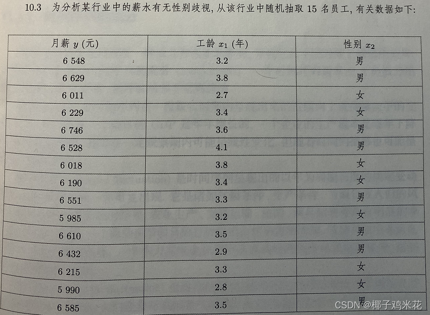
（1）

> example10_3<-read.csv("D:/作业/统计学R/《统计学—基于R》（第4版）—例题和习题数据（公开资源）/exercise/chap10/exercise10_3.csv")
> model1<-lm(月薪~工龄,data=example10_3)
> summary(model1)

Call:
lm(formula = 月薪 ~ 工龄, data = example10_3)

Residuals:
    Min      1Q  Median      3Q     Max 
-474.90 -152.54  -63.05  218.46  318.53 

Coefficients:
            Estimate Std. Error t value Pr(>|t|)    
(Intercept)   5249.7      587.1   8.941 6.48e-07 ***
工龄           327.2      173.3   1.887   0.0817 .  
---
Signif. codes:  0 ‘***’ 0.001 ‘**’ 0.01 ‘*’ 0.05 ‘.’ 0.1 ‘ ’ 1

Residual standard error: 248.4 on 13 degrees of freedom
Multiple R-squared:  0.2151,	Adjusted R-squared:  0.1547 
F-statistic: 3.562 on 1 and 13 DF,  p-value: 0.08165

回归结果显示，模型不显著，R2=21.51%，模型的拟合程度较差

（2）

引入哑变量，建立二元回归模型

> model2<-lm(月薪~工龄+性别,data=example10_3)
> summary(model2)

Call:
lm(formula = 月薪 ~ 工龄 + 性别, data = example10_3)

Residuals:
     Min       1Q   Median       3Q      Max 
-136.697  -67.380    1.351   54.888  154.863 

Coefficients:
            Estimate Std. Error t value Pr(>|t|)    
(Intercept)  6190.74     253.71  24.401 1.35e-11 ***
工龄          111.22      72.08   1.543    0.149    
性别女       -458.68      53.46  -8.580 1.82e-06 ***
---
Signif. codes:  0 ‘***’ 0.001 ‘**’ 0.01 ‘*’ 0.05 ‘.’ 0.1 ‘ ’ 1

Residual standard error: 96.79 on 12 degrees of freedom
Multiple R-squared:   0.89,	Adjusted R-squared:  0.8717 
F-statistic: 48.54 on 2 and 12 DF,  p-value: 1.773e-06

引入哑变量后，模型显著，Ra2=87.17%，模型的拟合程度大幅提高，表示有必要引入哑变量

（3）

用Anova方法比较模型：

> anova(model2,model1)
Analysis of Variance Table

Model 1: 月薪 ~ 工龄 + 性别
Model 2: 月薪 ~ 工龄
  Res.Df    RSS Df Sum of Sq     F    Pr(>F)    
1     12 112423                                 
2     13 802137 -1   -689714 73.62 1.823e-06 ***
---
Signif. codes:  0 ‘***’ 0.001 ‘**’ 0.01 ‘*’ 0.05 ‘.’ 0.1 ‘ ’ 1

用AIC方法比较模型：

> AIC(model2,model1)
       df      AIC
model2  4 184.3978
model1  3 211.8729

比较结果显示，引入性别哑变量模型比不引入性别哑变量模型差异显著，AIC也较小，表示有必要引入哑变量

本次记录就到这~~

椰子鸡米花

关注

10
点赞
踩
50

收藏

觉得还不错? 一键收藏
0
评论
2021-12-16 统计学-基于R（第四版）第十章课后习题记录及总结

先声明，本博客为个人作业不一定为标准答案，仅供参考10.1 题目如下（1）> example10_1<-read.csv("D:/作业/统计学R/《统计学—基于R》（第4版）—例题和习题数据（公开资源）/exercise/chap10/exercise10_1.csv")> model1<-lm(不良贷款~贷款余额+应收贷款+贷款项目个数+固定资产投资,data=example10_1)> summary(model1)Call:lm(for..
复制链接

扫一扫