2021-12-23 统计学-基于R（第四版）第十一章课后习题记录及总结

最新推荐文章于 2022-04-21 11:44:50 发布

椰子鸡米花

最新推荐文章于 2022-04-21 11:44:50 发布

阅读量1.5k

点赞数 3

分类专栏： R语言学习文章标签： r语言统计学

本文链接：https://blog.csdn.net/m0_52461904/article/details/122105941

版权

R语言学习专栏收录该内容

14 篇文章 129 订阅

订阅专栏

先声明，本博客为个人作业不一定为标准答案，仅供参考

11.1 题目如下

（1）

m=5和m=10的平滑结果：

> example11_1<-read.csv("D:/作业/统计学R/《统计学—基于R》（第4版）—例题和习题数据（公开资源）/exercise/chap11/exercise11_1.csv")
> example11_1<-ts(example11_1,start=1)
> library(DescTools)
> ma5<-MoveAvg(example11_1[,2],order=5,align="center",endrule="keep")
> ma10<-MoveAvg(example11_1[,2],order=10,align="center",endrule="NA")
> data.frame(时间=example11_1[,1],收盘价格=example11_1[,2],ma5,ma10)
   时间 收盘价格    ma5    ma10
1     1    33.82 33.820      NA
2     2    33.64 33.640      NA
3     3    34.00 33.964      NA
4     4    34.09 34.054      NA
5     5    34.27 34.126      NA
6     6    34.27 34.090 33.9505
7     7    34.00 34.054 33.9230
8     8    33.82 33.964 33.8770
9     9    33.91 33.820 33.7995
10   10    33.82 33.692 33.6905
11   11    33.55 33.600 33.5455
12   12    33.36 33.454 33.3915
13   13    33.36 33.290 33.2600
14   14    33.18 33.108 33.1420
15   15    33.00 32.946 33.0145
16   16    32.64 32.802 32.8865
17   17    32.55 32.712 32.7590
18   18    32.64 32.602 32.6050
19   19    32.73 32.546 32.4645
20   20    32.45 32.436 32.3780
21   21    32.36 32.236 32.3320
22   22    32.00 32.108 32.3085
23   23    31.64 32.090 32.2990
24   24    32.09 32.090 32.2990
25   25    32.36 32.162 32.2990
26   26    32.36 32.362 32.3035
27   27    32.36 32.490 32.3215
28   28    32.64 32.508 32.3710
29   29    32.73 32.526 32.4525
30   30    32.45 32.508 32.5390
31   31    32.45 32.452      NA
32   32    32.27 32.506      NA
33   33    32.36 32.652      NA
34   34    33.00 33.000      NA
35   35    33.18 33.180      NA

图形比较如下：

> plot(example11_1[,2],type='o',xlab="时间",ylab="收盘价格")
> lines(ma5,type='o',lty=2,col="red")
> lines(ma10,type='o',lty=6,col="blue")
> legend(x="topright",legend=c("收盘价格","ma5","ma10"),lty=c(1,2,6),col=c("black","red","blue"),fill=c(1,2,4),cex=0.8)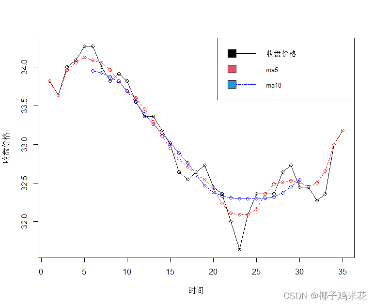

（2）

（a）

简单指数平滑预测：

> cpiforecast<-HoltWinters(example11_1[,2],beta=FALSE,gamma=FALSE)
> cpiforecast$fitted
Time Series:
Start = 2 
End = 35 
Frequency = 1 
       xhat    level
 2 33.82000 33.82000
 3 33.64001 33.64001
 4 33.99998 33.99998
 5 34.09000 34.09000
 6 34.26999 34.26999
 7 34.27000 34.27000
 8 34.00001 34.00001
 9 33.82001 33.82001
10 33.91000 33.91000
11 33.82000 33.82000
12 33.55001 33.55001
13 33.36001 33.36001
14 33.36000 33.36000
15 33.18001 33.18001
16 33.00001 33.00001
17 32.64002 32.64002
18 32.55000 32.55000
19 32.64000 32.64000
20 32.73000 32.73000
21 32.45001 32.45001
22 32.36000 32.36000
23 32.00002 32.00002
24 31.64002 31.64002
25 32.08998 32.08998
26 32.35999 32.35999
27 32.36000 32.36000
28 32.36000 32.36000
29 32.63999 32.63999
30 32.73000 32.73000
31 32.45001 32.45001
32 32.45000 32.45000
33 32.27001 32.27001
34 32.36000 32.36000
35 32.99997 32.99997

简单指数平滑拟合图：

> plot(example11_1[,2],type='o',xlab="时间",ylab="收盘价格")
> lines(example11_1[,1][-1],cpiforecast$fitted[,1],type='o',lty=2,col="blue")
> legend(x="topright",legend=c("观测值","拟合值"),lty=1:2,col=c(1,4),fill=c("black","blue"),cex=0.8)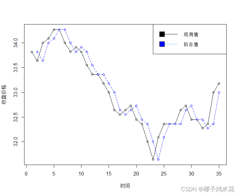

简单指数平滑下一期预测值：

> library(forecast)
> cpiforecast1<-forecast(cpiforecast,h=1)
> cpiforecast1
   Point Forecast    Lo 80    Hi 80    Lo 95   Hi 95
36       33.17999 32.87182 33.48816 32.70869 33.6513

简单指数平滑预测图：

> plot(cpiforecast1,type='o',xlab="时间",ylab="收盘价格",main="简单指数平滑预测")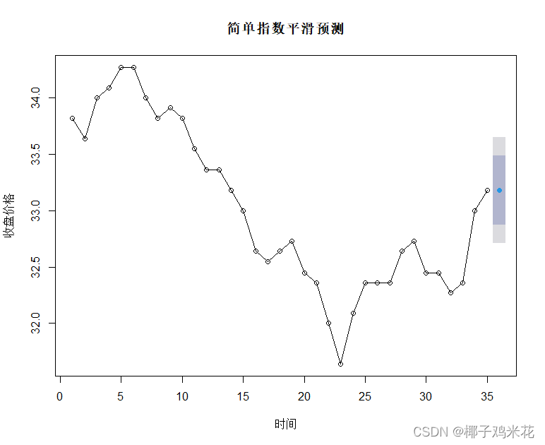

（灰色区域是预测值的置信区间，浅灰色为95%置信区间，深灰色为80%置信区间）

Holt指数平滑预测：

> powerforecast<-HoltWinters(example11_1[,2],gamma=FALSE)
> powerforecast$fitted
Time Series:
Start = 3 
End = 35 
Frequency = 1 
       xhat level       trend
 3 33.46000 33.64 -0.18000000
 4 33.89869 34.00 -0.10131106
 5 34.01657 34.09 -0.07343316
 6 34.23350 34.27 -0.03650281
 7 34.23882 34.27 -0.03118361
 8 33.93402 34.00 -0.06598400
 9 33.73740 33.82 -0.08259844
10 33.85255 33.91 -0.05744735
11 33.75781 33.82 -0.06219093
12 33.45753 33.55 -0.09247292
13 33.25332 33.36 -0.10668460
14 33.26886 33.36 -0.09113849
15 33.07591 33.18 -0.10408741
16 32.88485 33.00 -0.11514941
17 32.48917 32.64 -0.15082911
18 32.40803 32.55 -0.14196507
19 32.53184 32.64 -0.10816306
20 32.65071 32.73 -0.07928669
21 32.34147 32.45 -0.10853468
22 32.25417 32.36 -0.10583381
23 31.85713 32.00 -0.14287097
24 31.46549 31.64 -0.17451107
25 32.00649 32.09 -0.08350715
26 32.32801 32.36 -0.03199400
27 32.33267 32.36 -0.02733182
28 32.33665 32.36 -0.02334902
29 32.66086 32.64  0.02085508
30 32.76093 32.73  0.03093089
31 32.43562 32.45 -0.01437804
32 32.43772 32.45 -0.01228287
33 32.23328 32.27 -0.03672265
34 32.34174 32.36 -0.01825659
35 33.07766 33.00  0.07766473

Holt指数平滑拟合图：

> plot(example11_1[,2],type='o',xlab="时间",ylab="收盘价格")
> lines(example11_1[,1][c(-1,-2)],powerforecast$fitted[,1],type='o',lty=2,col="blue")
> legend(x="topright",legend=c("观测值","拟合值"),lty=1:2,col=c(1,4),fill=c("black","blue"),cex=0.8)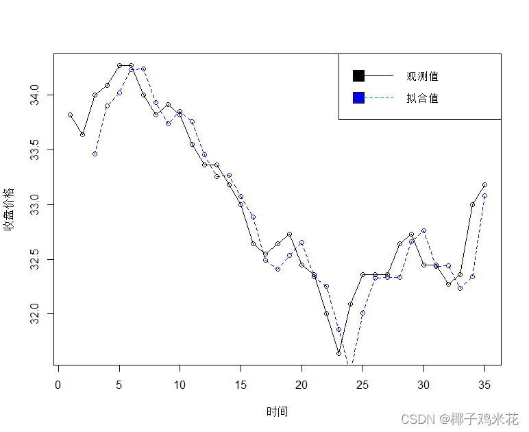

Holt指数平滑下一期预测值：

> powerforecast1<-forecast(powerforecast,h=1)
> powerforecast1
   Point Forecast    Lo 80    Hi 80   Lo 95    Hi 95
36       33.27258 32.95429 33.59086 32.7858 33.75935

Holt指数平滑预测图：

> plot(powerforecast1,type='o',xlab="时间",ylab="收盘价格",main="Holt指数平滑预测")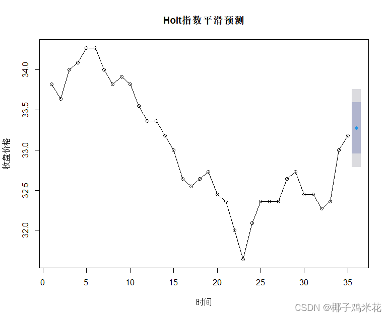

简单指数和Holt指数预测的残差比较：

> example11_1<-read.csv("D:/作业/统计学R/《统计学—基于R》（第4版）—例题和习题数据（公开资源）/exercise/chap11/exercise11_1.csv")
> example11_1<-ts(example11_1,start=1)
> library(forecast)
> cpiforecast<-HoltWinters(example11_1[,2],beta=FALSE,gamma=FALSE)
> cpiforecast1<-forecast(cpiforecast,h=1)
> powerforecast1<-forecast(powerforecast,h=1)
> residual1<-cpiforecast1$residuals
> residual2<-powerforecast1$residuals
> plot(as.numeric(residual1),pch=1,ylim=c(-1,1),xlim=c(0,40),xlab="时间",ylab="收盘价格")
> points(residual2,pch=19,col="blue")
> abline(h=0,lty=2,col=2)
> legend(x="topright",legend=c("简单指数预测残差","Holt指数预测残差"),pch=c(1,19),col=c("black","blue"),cex=1)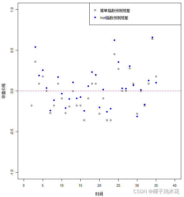

（b）

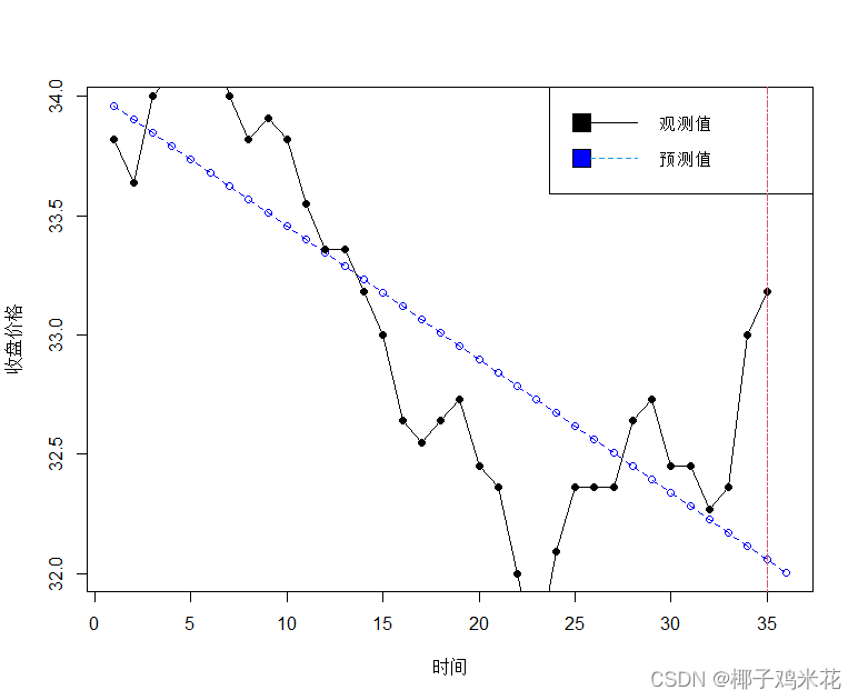
一元线性回归预测值：

> example11_1<-read.csv("D:/作业/统计学R/《统计学—基于R》（第4版）—例题和习题数据（公开资源）/exercise/chap11/exercise11_1.csv")
> fit<-lm(收盘价格~时间,data=example11_1)
> predata<-predict(fit,data.frame(时间=1:36))
> predata
       1        2        3        4        5        6        7        8        9       10 
33.95995 33.90407 33.84819 33.79231 33.73643 33.68055 33.62468 33.56880 33.51292 33.45704 
      11       12       13       14       15       16       17       18       19       20 
33.40116 33.34528 33.28940 33.23352 33.17764 33.12176 33.06588 33.01000 32.95412 32.89824 
      21       22       23       24       25       26       27       28       29       30 
32.84236 32.78648 32.73060 32.67472 32.61884 32.56296 32.50708 32.45120 32.39532 32.33945 
      31       32       33       34       35       36 
32.28357 32.22769 32.17181 32.11593 32.06005 32.00417

一元线性回归预测图：

> plot(1:36,predata,type='o',lty=2,col="blue",xlab="时间",ylab="收盘价格")
> lines(example11_1[,1],example11_1[,2],type='o',pch=19)
> legend(x="topright",legend=c("观测值","预测值"),lty=1:2,col=c(1,4),fill=c("black","blue"),cex=0.8)
> abline(v=35,lty=6,col=2)

指数预测值：

> example11_1<-read.csv("D:/作业/统计学R/《统计学—基于R》（第4版）—例题和习题数据（公开资源）/exercise/chap11/exercise11_1.csv")
> example11_1<-ts(example11_1,start=1)
> y<-log(example11_1[,2])
> x<-1:35
> fit<-lm(y~x)
> predata<-exp(predict(fit,data.frame(x=1:36)))
> predata
       1        2        3        4        5        6        7        8 
33.96096 33.90380 33.84673 33.78976 33.73288 33.67610 33.61942 33.56283 
       9       10       11       12       13       14       15       16 
33.50633 33.44993 33.39363 33.33742 33.28131 33.22529 33.16936 33.11353 
      17       18       19       20       21       22       23       24 
33.05779 33.00215 32.94660 32.89114 32.83578 32.78051 32.72533 32.67025 
      25       26       27       28       29       30       31       32 
32.61526 32.56036 32.50555 32.45084 32.39622 32.34169 32.28725 32.23290 
      33       34       35       36 
32.17865 32.12448 32.07041 32.01643

指数预测图：

> plot(1:36,predata,type='o',lty=2,col="blue",xlab="时间",ylab="收盘价格")
> points(example11_1[,1],example11_1[,2],type='o',pch=19)
> legend(x="topright",legend=c("观测值","预测值"),lty=1:2,col=c(1,4),fill=c("black","blue"),cex=0.8)
> abline(v=35,lty=6,col=2)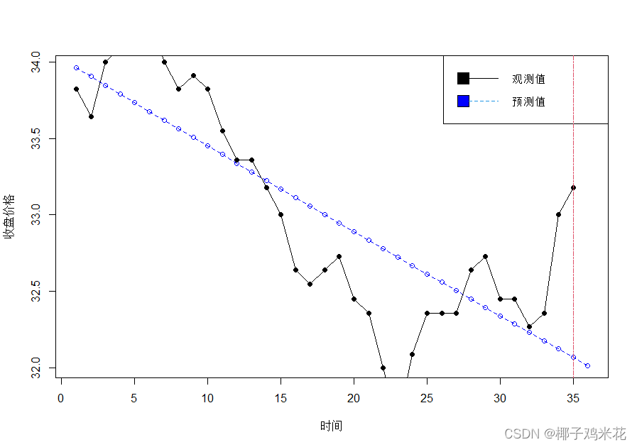

一元线性回归预测和指数预测的残差比较：

> example11_1<-read.csv("D:/作业/统计学R/《统计学—基于R》（第4版）—例题和习题数据（公开资源）/exercise/chap11/exercise11_1.csv")
> example11_1<-ts(example11_1,start=1)
> fit1<-lm(收盘价格~时间,data=example11_1)
> y<-log(example11_1[,2])
> x<-1:35
> fit2<-lm(y~x)
> predata2<-exp(predict(fit2,data.frame(x=1:36)))
> predata2<-ts(predata2,start=1)
> residual2<-example11_1[,2]-predata2
> residual1<-fit1$residuals
> plot(as.numeric(residual1),pch=1,ylim=c(-1,1),xlim=c(0,40),xlab="时间",ylab="收盘价格")
> points(residual2,pch=19,col="blue")
> legend(x="topright",legend=c("一元线性回归预测残差","指数预测残差"),pch=c(1,19),col=c("black","blue"),cex=1)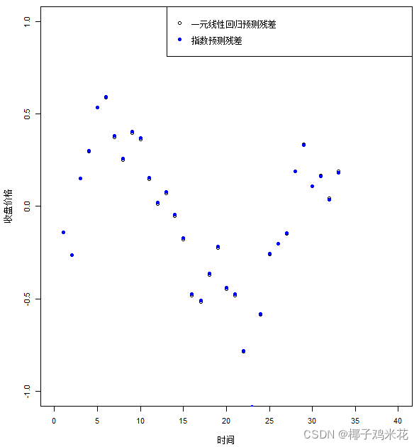

（c）

二阶曲线预测：

> example11_1<-read.csv("D:/作业/统计学R/《统计学—基于R》（第4版）—例题和习题数据（公开资源）/exercise/chap11/exercise11_1.csv")
> y<-example11_1[,2]
> x<-1:35
> fit1<-lm(y~x+I(x^2))
> predata1<-predict(fit1,data.frame(x=1:36))
> predata1
       1        2        3        4        5        6        7        8 
34.53224 34.37537 34.22462 34.07999 33.94148 33.80909 33.68282 33.56267 
       9       10       11       12       13       14       15       16 
33.44865 33.34074 33.23896 33.14329 33.05375 32.97033 32.89303 32.82185 
      17       18       19       20       21       22       23       24 
32.75678 32.69784 32.64503 32.59833 32.55775 32.52329 32.49496 32.47274 
      25       26       27       28       29       30       31       32 
32.45664 32.44667 32.44282 32.44508 32.45347 32.46798 32.48861 32.51536 
      33       34       35       36 
32.54823 32.58722 32.63233 32.68356

三阶曲线预测：

> example11_1<-read.csv("D:/作业/统计学R/《统计学—基于R》（第4版）—例题和习题数据（公开资源）/exercise/chap11/exercise11_1.csv")
> y<-example11_1[,2]
> x<-1:35
> fit2<-lm(y~x+I(x^2)+I(x^3))
> predata2<-predict(fit2,data.frame(x=1:36))
> predata2
       1        2        3        4        5        6        7        8 
33.94676 33.99653 34.02111 34.02246 34.00253 33.96329 33.90668 33.83467 
       9       10       11       12       13       14       15       16 
33.74922 33.65227 33.54579 33.43173 33.31205 33.18871 33.06366 32.93886 
      17       18       19       20       21       22       23       24 
32.81627 32.69784 32.58554 32.48131 32.38711 32.30491 32.23666 32.18431 
      25       26       27       28       29       30       31       32 
32.14982 32.13515 32.14225 32.17309 32.22961 32.31378 32.42756 32.57289 
      33       34       35       36 
32.75174 32.96606 33.21781 33.50895

二阶曲线和三阶曲线预测图：

> plot(1:36,predata2,type='o',lty=2,col="red",xlab="时间",ylab="收盘价格",main="二阶曲线和三阶曲线预测图")
> lines(1:36,predata1,type='o',lty=3,col="blue")
> points(example11_1[,1],example11_1[,2],type='o',pch=19)
> legend(x="bottomleft",legend=c("观测值","二阶曲线","三阶曲线"),lty=1:3,col=c("black","blue","red"),fill=c("black","blue","red"))
> abline(v=35,lty=6,col=2)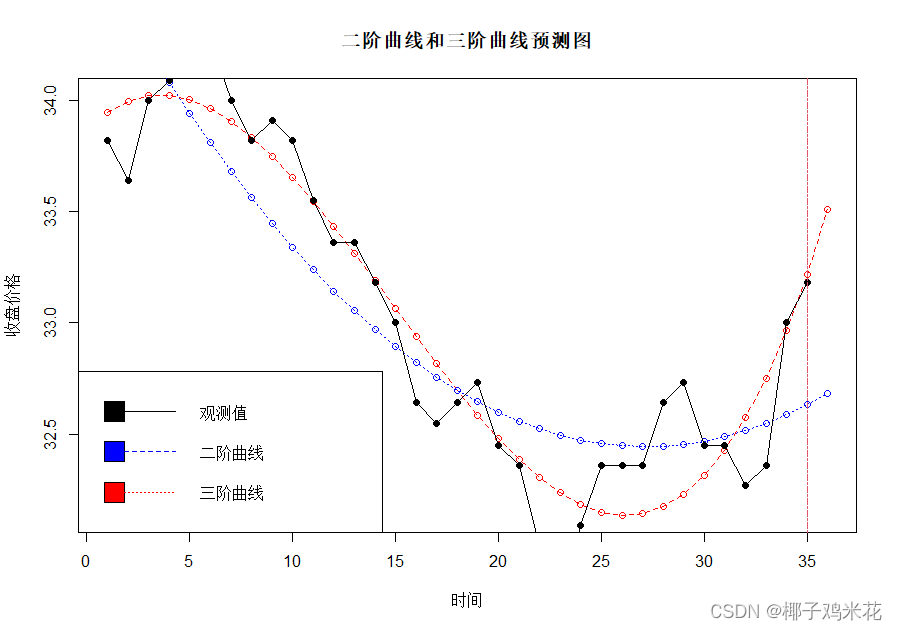

二阶曲线和三阶曲线预测的残差比较：

> example11_1<-read.csv("D:/作业/统计学R/《统计学—基于R》（第4版）—例题和习题数据（公开资源）/exercise/chap11/exercise11_1.csv")
> y<-example11_1[,2]
> x<-1:35
> fit1<-lm(y~x+I(x^2))
> fit2<-lm(y~x+I(x^2)+I(x^3))
> plot(fit1$residuals,pch=1,ylim=c(-1,1),xlim=c(0,40),xlab="时间",ylab="收盘价格")
> points(fit2$residuals,pch=19,col="blue")
> legend(x="topright",legend=c("二阶曲线预测残差","三阶曲线预测残差"),pch=c(1,19),col=c("black","blue"),cex=1)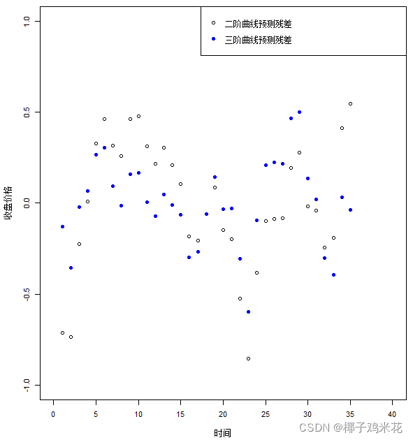

11.2 题目如下

（1）

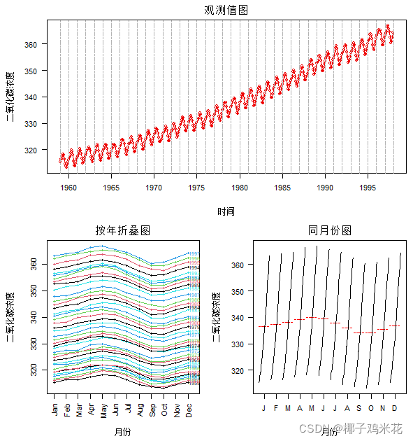
观测值图、按年折叠图、同月份图：

> library(reshape2)
> library(forecast)
> df<-melt(co2,variable.name="年份",value.name = "二氧化碳浓度")
> df.ts<-ts(df[,1],start=1959,frequency=12)
> layout(matrix(c(1,1,2,3),nrow=2,ncol=2,byrow=TRUE))
> par(mai=c(0.7,0.7,0.3,0.1),las=1,mgp=c(3.5,1,0),lab=c(6,6,1),cex=0.7,cex.lab=1,font.main=1)
> plot(df.ts,type='o',col="red2",xlab="时间",ylab="二氧化碳浓度",main="观测值图")
> abline(v=c(1959:1998),lty=6,col="gray70")
> par(las=3)
> seasonplot(df.ts,col=1:5,xlab="月份",ylab="二氧化碳浓度",main="按年折叠图",year.labels=TRUE,cex=0.6)
> par(las=1)
> monthplot(df.ts,xlab="月份",ylab="二氧化碳浓度",lty.base=6,col.base="red",cex=0.8,main="同月份图")

（2）

Winter指数平滑预测：

观测值和拟合值图：

> saleforecast<-HoltWinters(df.ts)
> plot(df.ts,type='o',col="grey40",xlab="年份",ylab="二氧化碳浓度")
> lines(saleforecast$fitted[,1],type='o',lty=5,col="blue")
> legend(x="topleft",legend=c("观测值","拟合值"),lty=c(1,5),col=c(1,4),fill=c(1,4))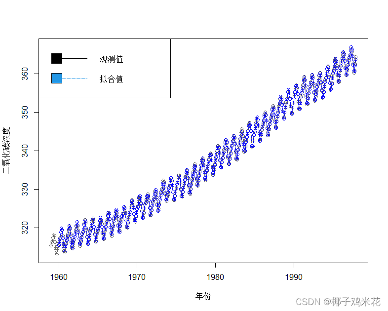

1998年和1999年的预测值：

> library(forecast)
> saleforecast1<-forecast(saleforecast,h=24)
> saleforecast1
         Point Forecast    Lo 80    Hi 80    Lo 95    Hi 95
Jan 1998       365.1079 364.7139 365.5019 364.5053 365.7105
Feb 1998       365.9664 365.5228 366.4100 365.2879 366.6449
Mar 1998       366.7343 366.2453 367.2234 365.9864 367.4823
Apr 1998       368.1364 367.6051 368.6678 367.3238 368.9490
May 1998       368.6674 368.0961 369.2386 367.7937 369.5410
Jun 1998       367.9508 367.3416 368.5599 367.0192 368.8824
Jul 1998       366.5318 365.8863 367.1772 365.5446 367.5189
Aug 1998       364.3799 363.6995 365.0604 363.3392 365.4206
Sep 1998       362.4731 361.7587 363.1874 361.3806 363.5656
Oct 1998       362.7520 362.0048 363.4993 361.6093 363.8948
Nov 1998       364.2203 363.4411 364.9996 363.0285 365.4121
Dec 1998       365.6741 364.8636 366.4847 364.4345 366.9138
Jan 1999       366.6048 365.7349 367.4747 365.2744 367.9353
Feb 1999       367.4633 366.5643 368.3623 366.0884 368.8383
Mar 1999       368.2313 367.3036 369.1590 366.8125 369.6500
Apr 1999       369.6333 368.6774 370.5893 368.1713 371.0954
May 1999       370.1643 369.1804 371.1482 368.6596 371.6690
Jun 1999       369.4477 368.4363 370.4592 367.9008 370.9946
Jul 1999       368.0287 366.9900 369.0674 366.4401 369.6173
Aug 1999       365.8769 364.8111 366.9426 364.2469 367.5068
Sep 1999       363.9700 362.8775 365.0625 362.2991 365.6409
Oct 1999       364.2490 363.1299 365.3680 362.5375 365.9604
Nov 1999       365.7172 364.5718 366.8626 363.9655 367.4690
Dec 1999       367.1710 365.9995 368.3426 365.3793 368.9628

预测图：

> plot(saleforecast1,xlab="年份",ylab="二氧化碳浓度",main="Winter模型的预测图")
> abline(v=1998,lty=6,col=2)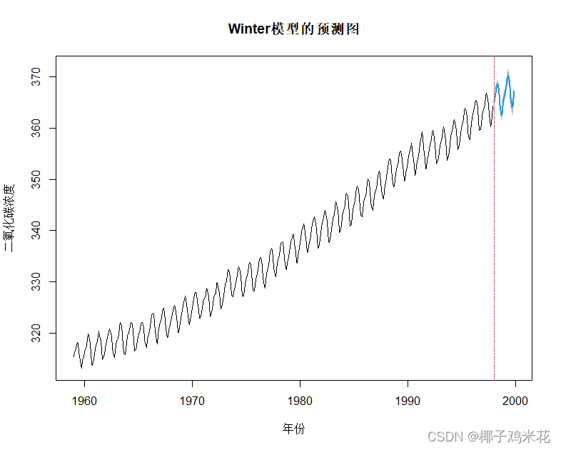

分解法预测：

成分分解图：

> library(reshape2)
> df<-melt(co2,variable.name="年份",value.name = "二氧化碳浓度")
> df.ts<-ts(df[,1],start=1959,frequency=12)
> salecompose<-decompose(df.ts,type="multiplicative")
> plot(salecompose,type='o',col="red4")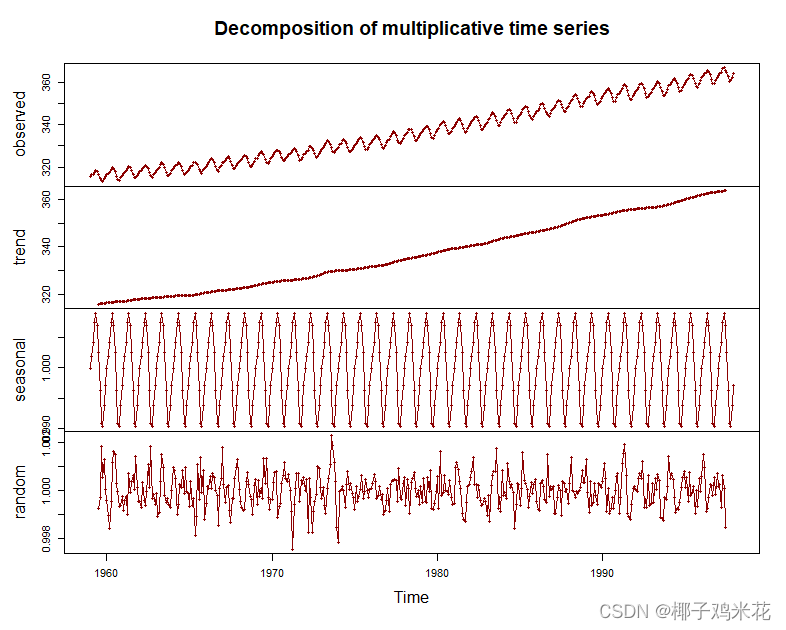

1998年和1999年各月份的预测值：

> seasonaladjust<-co2/salecompose$seasonal
> x<-1:length(seasonaladjust)
> fit<-lm(seasonaladjust~x)
> predata<-predict(fit,data.frame(x=469:492))*rep(salecompose$seasonal[1:12],1)
> predata<-ts(predata,start=1998,frequency = 12)
> predata
          Jan      Feb      Mar      Apr
1998 362.6057 363.4286 364.3609 365.6973
1999 363.9160 364.7414 365.6767 367.0176
          May      Jun      Jul      Aug
1998 366.3293 365.7196 364.2036 362.0834
1999 367.6515 367.0391 365.5173 363.3890
          Sep      Oct      Nov      Dec
1998 360.2463 360.1374 361.5225 362.8225
1999 361.5449 361.4353 362.8249 364.1292

（x=469:492，469为从length(seasonaladjust)后一位开始，492为468+12*2即后两年）

绘制观测值和观测值图：

> predata<-predict(fit,data.frame(x=1:492))*rep(salecompose$seasonal[1:12],1)
> predata<-ts(predata,start=1959,frequency = 12)
> plot(predata,type='o',lty=2,col="blue",xlab="年份",ylab="二氧化碳浓度")
> plot(predata,lty=2,col="blue",xlab="年份",ylab="二氧化碳浓度")
> lines(df.ts)
> legend(x="topleft",legend=c("观测值","预测值"),lty=1:2,col=c("black","blue"),fill=c("black","blue"))
> abline(v=1998,lty=6,col=2)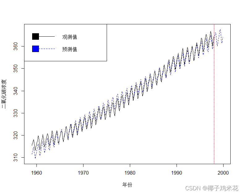

Winter模型预测与分解模型预测残差的比较：

> residuals1<-df.ts-predict(fit,data.frame(x=1:468))*salecompose$seasonal
> saleforecast<-HoltWinters(df.ts)
> residuals2<-df.ts-saleforecast$fitted[,1]
> plot(as.numeric(residuals1),pch=1,ylim=c(-4,4),xlab="时间",ylab="残差")
> points(as.numeric(residuals2),pch=19,col="blue")
> abline(h=0,lty=2,col=2)
> legend(x="topright",legend=c("分解预测残差","Winter模型预测残差"),pch=c(1,16),col=c("black","blue"),cex=0.7)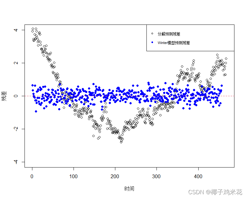

（这个图看上去有点奇怪不知道是不是哪里不对，但我目前没有找到不对的地方，如有错误请告知一下）

本次记录就到这，如有错误可指出~~画好多图啊！！

椰子鸡米花

关注

3
点赞
踩
14

收藏

觉得还不错? 一键收藏
0
评论
2021-12-23 统计学-基于R（第四版）第十一章课后习题记录及总结

先声明，本博客为个人作业不一定为标准答案，仅供参考11.1 题目如下（1）m=5和m=10的平滑结果：> example11_1<-read.csv("D:/作业/统计学R/《统计学—基于R》（第4版）—例题和习题数据（公开资源）/exercise/chap11/exercise11_1.csv")> example11_1<-ts(example11_1,start=1)> library(DescTools)> ma5<-MoveA.
复制链接

扫一扫