理解pytorch中的LSTM

pytroch中的LSTM

pytorch中的LSTM函数
pytorch中LSTM参数详解

以下是参数

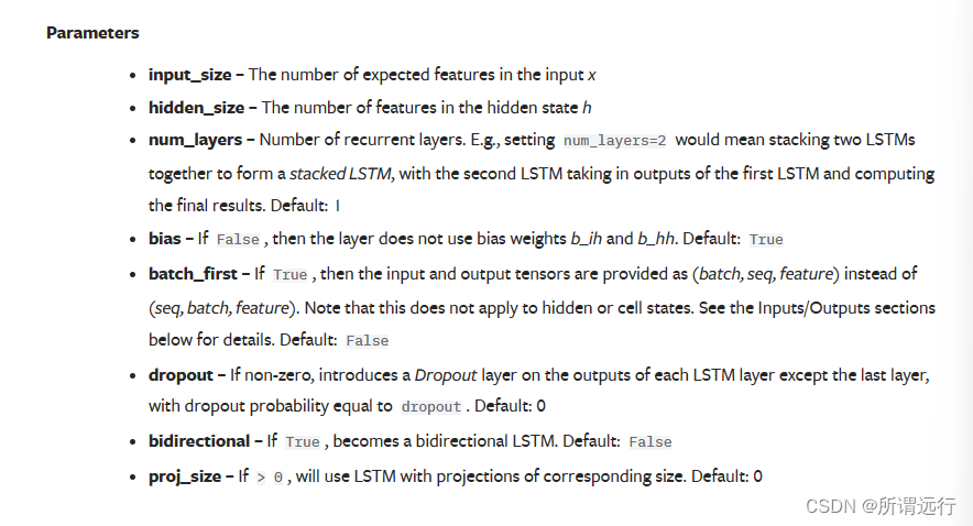
• input_size 输入节点维数
• hidden_size 隐藏节点个数
• num_layers 层数，

对于输入x的shape要求为x : [seq_length, batch_size, input_size]，理解这三个参数，可以参考用「动图」和「举例子」讲讲 RNN，这篇文章中：
介绍到RNN中时间步，time_step，每个t称为1步，t1 - t5为1个周期，RNN引入记忆概念，将上一个时间步产生的结果($Y_{t-1}$）同当前X一同输入进去。
理解time_step是神经网络的参数，网络建好了便不会改变，batch是训练参数，在训练时可根据效果随时调整。

搭建训练一个LSTM模型

LSTM代码实现

使用正余弦函数构造时间序列，而正余弦函数之间成导数关系，通过输入正弦函数的值来预测余弦函数的值。
取正弦函数的值作为LSTM的输入，预测对应时间下余弦函数的值。1个输入神经元，1个输出神经元，16个隐藏神经元，

完整代码：

import numpy as np
import torch
from torch import nn
import matplotlib.pyplot as plt

定义model

class LSTMRNN(nn.Module):
    def __init__(self, input_size, hidden_size=1, output_size=1, num_layers=1):
        super().__init__()
        self.lstm = nn.LSTM(input_size, hidden_size, num_layers)
        self.forwardCalculation = nn.Linear(hidden_size, output_size)

    def forward(self, _x):
        '''

        :param _x: input, (seq_len, batch, input_size)
        :return:
        '''
        x, _ = self.lstm(_x)
        s, b, h = x.shape
        x = x.view(s * b, h)  # view方法调整形状
        x = self.forwardCalculation(x)
        x = x.view(s, b, -1)  # 再次调整形状
        return x

定义数据

data_len = 200
t = np.linspace(0, 12 * np.pi, data_len)
sin_t = np.sin(t)
cos_t = np.cos(t)

# 创建一个全0的(data_len, 2)的数组，然后将sin和cos的值写进去
dataset = np.zeros((data_len, 2))  # 二维的数据
# print(dataset)
dataset[:, 0] = sin_t  # 第一列
dataset[:, 1] = cos_t
dataset = dataset.astype('float32')  # 调整类型
# print(dataset)
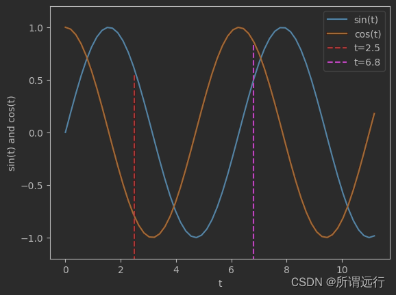
# 绘制一部分原始数据
plt.figure()
plt.plot(t[0:60], dataset[0:60, 0], label='sin(t)')
plt.plot(t[0:60], dataset[0:60, 1], label='cos(t)')
plt.plot([2.5, 2.5], [-1.3, 0.55], 'r--', label='t=2.5')
plt.plot([6.8, 6.8], [-1.3, 0.85], 'm--', label='t=6.8')
plt.xlabel('t')  # 时间
plt.ylim(-1.2, 1.2)
plt.ylabel('sin(t) and cos(t)')
plt.legend(loc='upper right')
plt.show()

如图所示：

划分数据集

# 对dataset划分训练集和测试集，，80%训练
train_data_ratio = 0.5
train_data_len = int(data_len * train_data_ratio)
train_x = dataset[:train_data_len, 0]
train_y = dataset[:train_data_len, 1]
INPUT_FEATURES_NUM = 1
OUTPUT_FEATURES_NUM = 1
t_for_training = t[:train_data_len]
# 测试集
test_x = dataset[train_data_len:, 0]
test_y = dataset[train_data_len:, 1]
t_for_test = t[train_data_len:]

训练

# 进行训练
train_x_tensor = train_x.reshape(-1, 5, INPUT_FEATURES_NUM)  # 每一批次为5个，
train_y_tensor = train_y.reshape(-1, 5, OUTPUT_FEATURES_NUM)

# 转换为tensor
train_x_tensor = torch.from_numpy(train_x_tensor)
train_y_tensor = torch.from_numpy(train_y_tensor)
print(train_x_tensor)
print(train_x_tensor.shape)
lstm_model = LSTMRNN(INPUT_FEATURES_NUM, 16, output_size=OUTPUT_FEATURES_NUM, num_layers=1)
print('LSTM model:', lstm_model)
print('model.parameters:', lstm_model.parameters)

loss_fun = nn.MSELoss()
optimizer = torch.optim.Adam(lstm_model.parameters(), lr=1e-2)
max_epochs = 10000
for epoch in range(max_epochs):
    output = lstm_model(train_x_tensor)  # 传入的整个train_x_tensor
    loss = loss_fun(output, train_y_tensor)
    loss.backward()
    optimizer.step()
    optimizer.zero_grad()

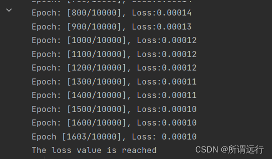
    if loss.item() < 1e-4:
        print('Epoch [{}/{}], Loss: {:.5f}'.format(epoch + 1, max_epochs, loss.item()))
        print("The loss value is reached")
        break
    elif (epoch + 1) % 100 == 0:
        print('Epoch: [{}/{}], Loss:{:.5f}'.format(epoch + 1, max_epochs, loss.item()))

训练过程：

查看预测结果

predictive_y_for_training = lstm_model(train_x_tensor)
print(predictive_y_for_training)
predictive_y_for_training = predictive_y_for_training.view(-1, OUTPUT_FEATURES_NUM).data.numpy()  # 装换成一维的
print(predictive_y_for_training)

测试集

# eval
lstm_model = lstm_model.eval()  # 转为测试
test_x_tensor = test_x.reshape(-1, 5, INPUT_FEATURES_NUM)
test_x_tensor = torch.from_numpy(test_x_tensor)
predictive_y_for_testing = lstm_model(test_x_tensor)
predictive_y_for_testing = predictive_y_for_testing.view(-1, OUTPUT_FEATURES_NUM).data.numpy()
print(predictive_y_for_testing)

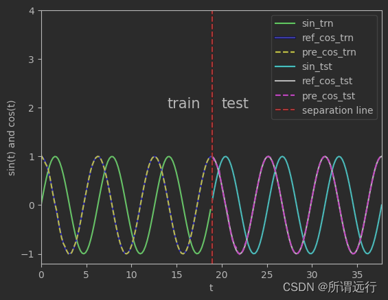
绘制

plt.figure()
plt.plot(t_for_training, train_x, 'g', label='sin_trn')
plt.plot(t_for_training, train_y, 'b', label='ref_cos_trn')
plt.plot(t_for_training, predictive_y_for_training, 'y--', label='pre_cos_trn')
plt.plot(t_for_test, test_x, 'c', label='sin_tst')
plt.plot(t_for_test, test_y, 'k', label='ref_cos_tst')
plt.plot(t_for_test, predictive_y_for_testing, 'm--', label='pre_cos_tst')

plt.plot([t[train_data_len], t[train_data_len]], [-1.2, 4.0], 'r--', label='separation line')  # separation line

plt.xlabel('t')
plt.ylabel('sin(t) and cos(t)')
plt.xlim(t[0], t[-1])
plt.ylim(-1.2, 4)
plt.legend(loc='upper right')
plt.text(14, 2, "train", size=15, alpha=1.0)
plt.text(20, 2, "test", size=15, alpha=1.0)

plt.show()

如图所示：

时间序列git:
https://github.com/microprediction/timeseries-notebooks/tree/main
https://github.com/cerlymarco/MEDIUM_NoteBook