NumPy的高级应用

NumPy的高级应用

import numpy as np
import pandas as pd
import matplotlib.pyplot as plt

plt.rcParams['font.sans-serif'] = ['SimHei']
plt.rcParams['axes.unicode_minus'] = False

%config InlineBackend.figure_format = 'svg'

import warnings

warnings.filterwarnings("ignore")

常用函数

• 联结

# 沿axis=1联结
np.hstack((array1, array2))

# 沿axis=0联结
np.vstack((array1, array2))

np.concatenate((array1, array2))

np.concatenate((array1, array2), axis=1)

• 拆分
  

# append会进行扁平化处理
np.append(array1, 10)
#array([ 1,  2,  3,  4,  5,  6,  7,  8,  9, 10])

# insert会进行扁平化处理
np.insert(array1, 0, 0)
# array([0, 1, 2, 3, 4, 5, 6, 7, 8, 9])

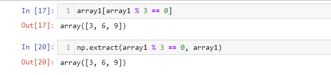
# 根据条件和公式获取数据
x = np.arange(10)
condlist = [x<3, x>5]
choicelist = [x, x**2]
np.select(condlist, choicelist, default=np.nan)

输出： array([ 0., 1., 2., nan, nan, nan, 36., 49., 64., 81.])

# 根据条件和公式获取数据
np.where(x < 5, x, 10*x)

输出：array([ 0, 1, 2, 3, 4, 50, 60, 70, 80, 90])

def fib(n):
    a, b = 0, 1
    for _ in range(n):
        a, b = b, a + b
        yield a
    
gen = fib(20)
array3 = np.fromiter(gen, dtype=np.int64, count=15)
array3

输出：array([ 1, 1, 2, 3, 5, 8, 13, 21, 34, 55, 89, 144, 233,377, 610],dtype=int64)

矩阵的运算

向量

点积运算

$$A\cdot B=a_1{b}_1+a_2{b}_2=|A||B|cos\theta$$$$A\cdot B=\sum _{i=1}^n{a}_i{b}_i=|A||B|cos\theta$$

数组的点积

1. 一维数组的点积
   • 计算公式：a[0] * b[0] +a[1] * b[1] +…+a[n]*b[n]
2. 二维数组的点积
   • C[0,0]=A[0,0] *B[0,0] + A[0,1] *B[1,0]：A的第一行与B的第一列，对应元素的乘积之和;
   • C[0,1]=A[0,0] *B[0,1] + A[0,1] *B[1,1]：A的第一行与B的第二列，对应元素的乘积之和;
   • C[1,0]=A[1,0] *B[0,0] + A[1,1] *B[1,0]：A的第二行与B的第一列，对应元素的乘积之和;
   • C[1,1]=A[1,1] *B[0,1] + A[1,1] *B[1,1]：A的第二行与B的第二列，对应元素的乘积之和;

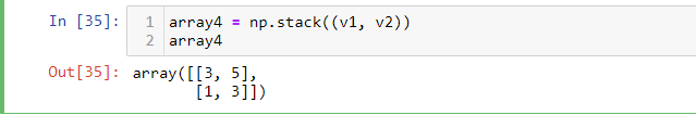
# 点积
v1 = np.array([3, 5])
v2 = np.array([1, 3])
np.dot(v1, v2)	# 18

# 叉积
np.outer(v1, v2)

输出：

# 求行列式
# linear algebra
np.linalg.det(array4).round(1)	# 4.0

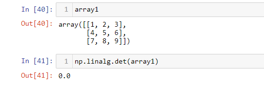
# 求矩阵的秩
np.linalg.matrix_rank(array1)	# 2

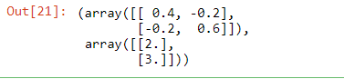
解线性方程

$$\{\begin{array}{l}3x+y=9\\ x+2y=8\end{array}$$$$\begin{gathered} Ax=b \\ {A}^{-1}Ax=A^{-1}b \\ Ix=A^{-1}b \end{gathered}$$

A = np.array([[3, 1], [1, 2]])
b = np.array([9, 8]).reshape(-1, 1)
# 求逆矩阵
A_1 = np.linalg.inv(A)
A_1, A_1 @ b

# 用solve求解
np.linalg.solve(A, b)

最小二乘解

# !pip install scikit-learn
from sklearn.datasets import load_boston

# 获取波士顿房价数据
dataset = load_boston()
print(dataset.DESCR) # 描述信息

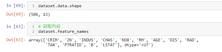
# 用波士顿房价数据创建DataFrame对象
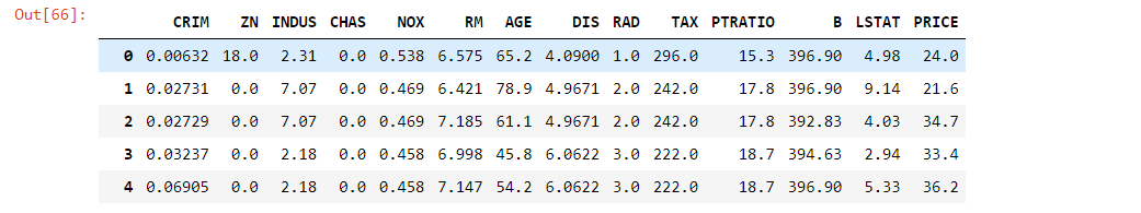
df = pd.DataFrame(data=dataset.data, columns=dataset.feature_names)
df.head(5) # 获取前五条数据

# 添加PRICE列
df['PRICE'] = dataset.target
df

# 协方差
df.cov()

# 皮尔逊相关系数(另外：kindall / spearman)
df.corr().round(2)

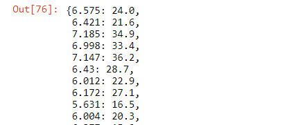
rooms = df['RM'].values
prices = df['PRICE'].values
history_data = { room: price for room, price in zip(rooms, prices)}
history_data

import heapq

nums = [35, 98, 76, 12, 55, 68, 47, 92]
# 获取前n大的值
print(heapq.nlargest(3, nums))
# 获取前n小的值
print(heapq.nsmallest(3, nums))

# KNN算法
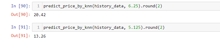
def predict_price_by_knn(history_data, room, k=5):
#     keys = sorted(history_data, key=lambda x: (x - room) ** 2)[:k]
    keys = heapq.nsmallest(k, history_data, key=lambda x: (x - room) ** 2)
    return np.mean([history_data[key] for key in keys])

plt.scatter(rooms, prices)
plt.show()
# plt.savefig('images/corr.svg')

损失函数：残差平方和 —> MSE
$$y=ax+b$$
$$MSE=\frac{1}{N}\sum (\widehat{y_i}-y_i{)}^2$$

def get_loss(a, b):
    """损失函数"""
    y_hat = a * rooms + b
    return np.mean((y_hat - prices) ** 2)

# 通过蒙特卡罗模拟(随机)找到最佳拟合的a和b的值
import random

best_a, best_b = None, None
min_loss = np.inf

for _ in range(1000):
    a = random.random() * 200 - 100
    b = random.random() * 200 - 100
    curr_loss = get_loss(a, b)
    if curr_loss < min_loss:
        min_loss = curr_loss
        best_a, best_b = a, b
print(best_a, best_b)
print(min_loss)

y_hat = 10.271 * rooms - 40.848

plt.scatter(rooms, prices)
plt.plot(rooms, y_hat, color='red')
plt.show()

梯度下降

损失函数是凹函数，找到使函数最小的a和b的值，可以用下面的方法：
$$a^{\prime }=a+(-1)\times \frac{\partial loss(a,b)}{\partial a}\times \Delta$$$$b^{\prime }=b+(-1)\times \frac{\partial loss(a,b)}{\partial b}\times \Delta$$
对于求MSE的损失函数来说，可以用下面的公式计算偏导数：
$$f(a,b)=\frac{1}{N}\sum _{i=1}^N(y_i-(a{x}_i+b){)}^2$$$$\frac{\partial f(a,b)}{\partial a}=\frac{2}{N}\sum _{i=1}^N(-x_i{y}_i+x_i^{2}a+x_{i}b)$$ $$\frac{\partial f(a,b)}{\partial b}=\frac{2}{N}\sum _{i=1}^N(-y_i+x_{i}a+b)$$

def get_loss(x, y, a, b):
    """损失函数"""
    y_hat = a * x + b
    return np.mean((y_hat - y) ** 2)

# 求a的偏导数
def partial_a(x, y, a, b):
    return 2 * np.mean((y - a * x - b) * (-x))


# 求b的偏导数
def partial_b(x, y, a, b):
    return 2 * np.mean(-y + a * x + b)

# 通过梯度下降的方式向拐点逼近
# 这种方式能够更快的找到最佳拟合的a和b
# a和b的初始值可以随意设定，delta的值要足够小
a, b = 35, -35
delta = 0.01

for _ in range(100):
    a = a - partial_a(rooms, prices, a, b) * delta
    b = b - partial_b(rooms, prices, a, b) * delta
print(a, b)
print(get_loss(rooms, prices, a, b))

# 通过线性回归方程预测房价
def predict_price_by_regression(a, b, x):
    return a * x + b

# 预测房价
print(np.round(predict_price_by_regression(best_a, best_b, 6.25), 2)) # 23.35
print(np.round(predict_price_by_regression(a, b, 6.25), 2)) # 22.2

print(np.round(predict_price_by_regression(best_a, best_b, 5.12), 2)) # 11.74
print(np.round(predict_price_by_regression(a, b, 5.12), 2)) # 11.93

# 比较两条拟合曲线
y_hat1 = best_a * rooms + best_b
y_hat2 = a * rooms + b
plt.scatter(rooms, prices)
plt.plot(rooms, y_hat1, color='red', linewidth=4)
plt.plot(rooms, y_hat2, color='green', linewidth=4)
plt.show()

最小二乘解就是用已经得到的历史数据（x和y的值）找到能够最佳拟合这些历史数据的a和b。
$$y=ax+b$$对于上面的方程，相当于x是变量a的系数，1是变量b的系数。

lstsq函数参数说明

lstsq函数参数说明

lstsq函数的第一个参数是

第二个参数就是y，rcond参数暂时不管，直接设置为None。

lstsq函数返回值说明

lstsq函数返回的是一个四元组，四元组中的第一个元素就是要求解的方程的系数，四元组中的第二个元素是误差平方和。

# 比较两条拟合曲线
plt.scatter(rooms, prices)
# 梯度下降法给出的a和b预测出的房价
plt.plot(rooms, y_hat2, color='red', linewidth=4)
# lstsq函数给出的a和b预测出的房价
y_hat3 = a * rooms + b
plt.plot(rooms, y_hat3, color='green', linewidth=4)
plt.show()