- LightGBM在数据量大的时候,速度会明显比XGBOOST快,但XGBOOST的预测准确性会更高。
from sklearn.preprocessing import OneHotEncoder
from xgboost import XGBRegressor
history_data = df_replen_2[['mot', 'country', 'priority', 'cc', 'climate_count','shippingfrequency','isgreen', 'holiday_count','forwarder', 'dayofweek','ts_pu_hour', 'lt_pu_pod']]
feature_cols = ['mot', 'country', 'priority', 'cc', 'climate_count','shippingfrequency','isgreen', 'holiday_count','forwarder', 'dayofweek']
encoder = OneHotEncoder(sparse=False, handle_unknown='ignore')
encoder.fit(history_data[feature_cols])
history_data_encoded = pd.DataFrame(encoder.transform(history_data[feature_cols]))
feature_names = encoder.get_feature_names(feature_cols)
history_data_encoded["ts_pu_hour"] = history_data["ts_pu_hour"]
history_data_encoded["lt_pu_pod"] = history_data["lt_pu_pod"]
train_data = history_data_encoded.sample(frac=0.8, random_state=123)
test_data = history_data_encoded.drop(train_data.index)
xgb_model = XGBRegressor(n_estimators=100, learning_rate=0.1, max_depth=20, reg_alpha=9, reg_lambda=5, gamma=0.6)
xgb_model.fit(train_data.iloc[:, :-1], train_data.iloc[:, -1])
r2_score = xgb_model.score(test_data.iloc[:, :-1], test_data.iloc[:, -1])
print("R2 score on test data:", r2_score)
new_data = df_replen_open[['mot', 'country', 'priority', 'cc', 'climate_count','shippingfrequency','isgreen', 'holiday_count','forwarder', 'dayofweek','ts_pu_hour']]
new_data_encoded = pd.DataFrame(encoder.transform(new_data[feature_cols]))
new_data_encoded['ts_pu_hour'] = new_data['ts_pu_hour']
predictions = xgb_model.predict(new_data_encoded)
print("Predictions:", predictions)
R2 score on test data: 0.9287763507620541
Predictions: [19.772514   7.7723885  6.275913  ... 13.262593   5.5251946  5.3950086]
new_data = df_replen_2[['mot', 'country', 'priority', 'cc', 'climate_count','shippingfrequency','isgreen', 'holiday_count','forwarder', 'dayofweek','ts_pu_hour']]
new_data_encoded = pd.DataFrame(encoder.transform(new_data[feature_cols]))
new_data_encoded['ts_pu_hour'] = new_data["ts_pu_hour"]
predictions = xgb_model.predict(new_data_encoded)
df_replen_2['forecast_lt_pu_pod_xgb'] = pd.Series(predictions)
df_replen_open['forecast_lt_pu_pod_xgb'] = pd.Series(predictions)
import lightgbm as lgb
from sklearn.preprocessing import OneHotEncoder
from sklearn.model_selection import train_test_split
from sklearn.metrics import r2_score
history_data = df_replen_2[['mot', 'country', 'priority', 'cc', 'climate_count','shippingfrequency','isgreen', 'holiday_count','forwarder', 'dayofweek','ts_pu_hour', 'lt_pu_pod']]
feature_cols = ['mot', 'country', 'priority', 'cc', 'climate_count','shippingfrequency','isgreen', 'holiday_count','forwarder', 'dayofweek','ts_pu_hour']
encoder = OneHotEncoder(sparse=False, handle_unknown='ignore')
encoder.fit(history_data[feature_cols])
history_data_encoded = pd.DataFrame(encoder.transform(history_data[feature_cols]))
feature_names = encoder.get_feature_names(feature_cols)
history_data_encoded["ts_pu_hour"] = history_data["ts_pu_hour"]
history_data_encoded["lt_pu_pod"] = history_data["lt_pu_pod"]
train_data, test_data = train_test_split(history_data_encoded, test_size=0.2, random_state=123)
X_train = train_data.iloc[:, :-1]
y_train = train_data.iloc[:, -1]
X_test = test_data.iloc[:, :-1]
y_test = test_data.iloc[:, -1]
lgb_model = lgb.LGBMRegressor(n_estimators=100, learning_rate=0.05, max_depth=22, reg_alpha=9, reg_lambda=5, gamma=0.6)
lgb_model.fit(X_train, y_train)
y_pred = lgb_model.predict(X_test)
r2_score_lgb = r2_score(y_test, y_pred)
print("R2 score using LightGBM:", r2_score_lgb)
new_data = df_replen_open[['mot', 'country', 'priority', 'cc', 'climate_count','shippingfrequency','isgreen', 'holiday_count','forwarder', 'dayofweek','ts_pu_hour']]
new_data_encoded = pd.DataFrame(encoder.transform(new_data[feature_cols]))
new_data_encoded['ts_pu_hour'] = new_data['ts_pu_hour']
predictions_lgb = lgb_model.predict(new_data_encoded)
print("Predictions using LightGBM:", predictions_lgb)
[LightGBM] [Warning] Unknown parameter: gamma
R2 score using LightGBM: 0.8743557858040798
Predictions using LightGBM: [17.6757881   8.03650015  5.94436404 ... 11.29174144  5.99137554
  5.94436404]
new_data = df_replen_2[['mot', 'country', 'priority', 'cc', 'climate_count','shippingfrequency','isgreen', 'holiday_count','forwarder', 'dayofweek','ts_pu_hour']]
new_data_encoded = pd.DataFrame(encoder.transform(new_data[feature_cols]))
new_data_encoded['ts_pu_hour'] = new_data['ts_pu_hour']
predictions_lgb = lgb_model.predict(new_data_encoded)
df_replen_2['forecast_lt_pu_pod_lgb'] = pd.Series(predictions_lgb)
df_replen_2['xgb_accuracy'] = df_replen_2['lt_pu_pod'] - df_replen_2['forecast_lt_pu_pod_xgb']
df_replen_2['lgb_accuracy'] = df_replen_2['lt_pu_pod'] - df_replen_2['forecast_lt_pu_pod_lgb']
country_list = df_replen_2[df_replen_2['geo']=='LAS']['country'].unique()
for country in country_list:
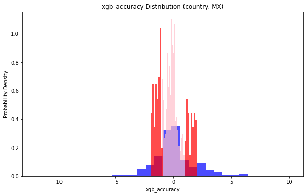
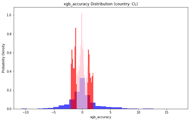
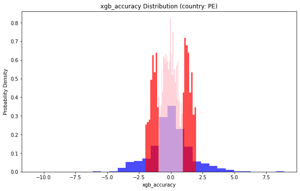
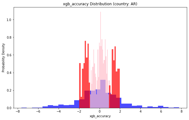
lt_pu_pod = df_replen_2[df_replen_2['country'] == country]['xgb_accuracy']
plt.figure(figsize=(10, 6))
plt.hist(lt_pu_pod, bins=30, density=True, alpha=0.7, color='b')
plt.hist(lt_pu_pod[np.abs(lt_pu_pod) < 1], bins=30, density=True, alpha=0.7, color='pink')
plt.hist(lt_pu_pod[(np.abs(lt_pu_pod) >= 1) & (np.abs(lt_pu_pod) < 2)], bins=30, density=True, alpha=0.7, color='red')
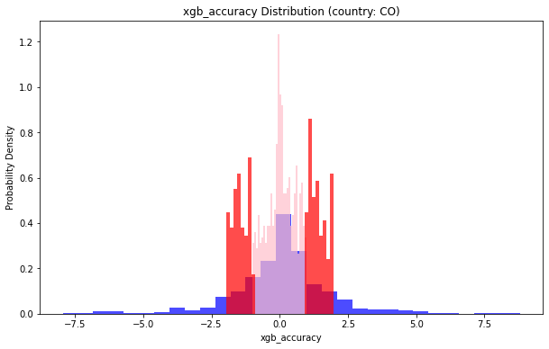
plt.title(f'xgb_accuracy Distribution (country: {country})')
plt.xlabel('xgb_accuracy')
plt.ylabel('Probability Density')
ratio_lt_1 = len(lt_pu_pod[np.abs(lt_pu_pod) < 1]) / len(lt_pu_pod)
ratio_lt_2 = len(lt_pu_pod[(np.abs(lt_pu_pod) >= 1) & (np.abs(lt_pu_pod) < 2)]) / len(lt_pu_pod)
print(f'地理位置(country: {country})小于1的部分占比:{ratio_lt_1}')
print(f'地理位置(country: {country})小于2的部分占比:{ratio_lt_2+ratio_lt_1}')
plt.show()
地理位置(country: MX)小于1的部分占比:0.5792474344355758
地理位置(country: MX)小于2的部分占比:0.7537058152793614
地理位置(country: CL)小于1的部分占比:0.5108045977011494
地理位置(country: CL)小于2的部分占比:0.7190804597701149
地理位置(country: PE)小于1的部分占比:0.5823324292909725
地理位置(country: PE)小于2的部分占比:0.8008523827973654
地理位置(country: AR)小于1的部分占比:0.45614035087719296
地理位置(country: AR)小于2的部分占比:0.7345029239766081
地理位置(country: CO)小于1的部分占比:0.5929791271347249
地理位置(country: CO)小于2的部分占比:0.8026565464895636
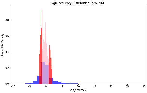
geo_list = df_replen_2['geo'].unique()
for geo in geo_list:
lt_pu_pod = df_replen_2[df_replen_2['geo'] == geo]['xgb_accuracy']
plt.figure(figsize=(10, 6))
plt.hist(lt_pu_pod, bins=30, density=True, alpha=0.7, color='b')
plt.hist(lt_pu_pod[np.abs(lt_pu_pod) < 1], bins=30, density=True, alpha=0.7, color='pink')
plt.hist(lt_pu_pod[(np.abs(lt_pu_pod) >= 1) & (np.abs(lt_pu_pod) < 2)], bins=30, density=True, alpha=0.7, color='red')
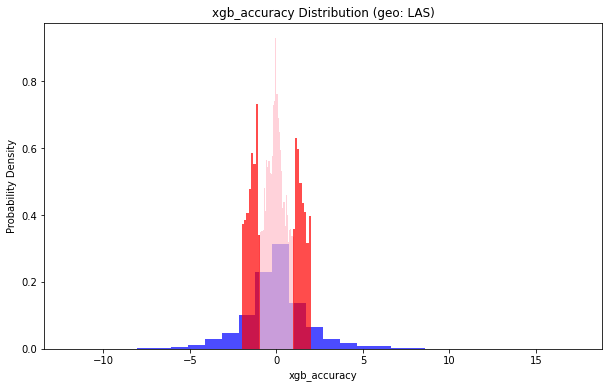
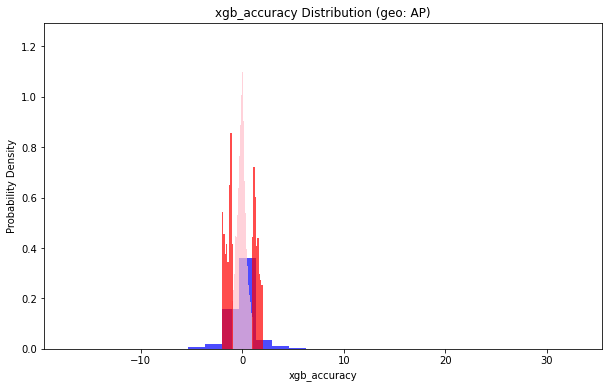
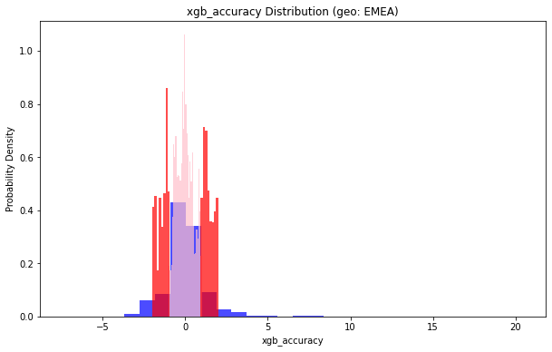
plt.title(f'xgb_accuracy Distribution (geo: {geo})')
plt.xlabel('xgb_accuracy')
plt.ylabel('Probability Density')
ratio_lt_1 = len(lt_pu_pod[np.abs(lt_pu_pod) < 1]) / len(lt_pu_pod)
ratio_lt_2 = len(lt_pu_pod[(np.abs(lt_pu_pod) >= 1) & (np.abs(lt_pu_pod) < 2)]) / len(lt_pu_pod)
print(f'地理位置(geo: {geo})小于1的部分占比:{ratio_lt_1}')
print(f'地理位置(geo: {geo})小于2的部分占比:{ratio_lt_2+ratio_lt_1}')
plt.show()
地理位置(geo: LAS)小于1的部分占比:0.5485282418456643
地理位置(geo: LAS)小于2的部分占比:0.7645186953062848
地理位置(geo: AP)小于1的部分占比:0.7526357962213225
地理位置(geo: AP)小于2的部分占比:0.8919323549257759
地理位置(geo: EMEA)小于1的部分占比:0.7375867592098239
地理位置(geo: EMEA)小于2的部分占比:0.9040754582665955
地理位置(geo: NA)小于1的部分占比:0.5368736150526766
地理位置(geo: NA)小于2的部分占比:0.7902266454146095
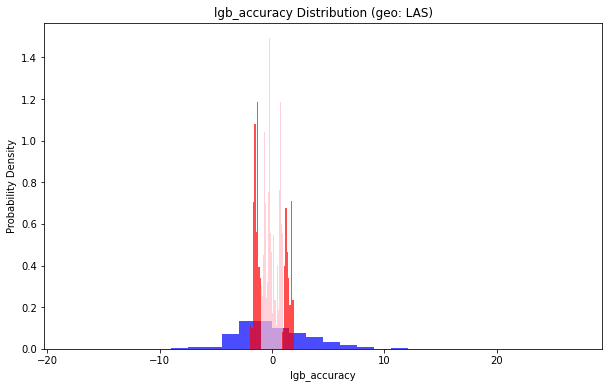
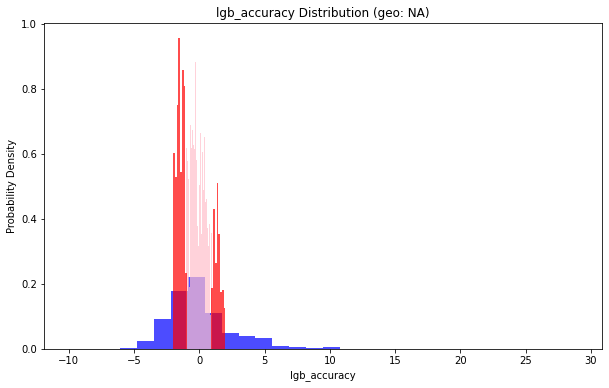
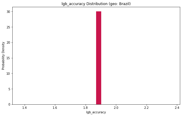
geo_list = df_replen_2['geo'].unique()
for geo in geo_list:
lt_pu_pod = df_replen_2[df_replen_2['geo'] == geo]['lgb_accuracy']
plt.figure(figsize=(10, 6))
plt.hist(lt_pu_pod, bins=30, density=True, alpha=0.7, color='b')
plt.hist(lt_pu_pod[np.abs(lt_pu_pod) < 1], bins=30, density=True, alpha=0.7, color='pink')
plt.hist(lt_pu_pod[(np.abs(lt_pu_pod) >= 1) & (np.abs(lt_pu_pod) < 2)], bins=30, density=True, alpha=0.7, color='red')
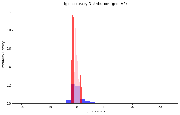
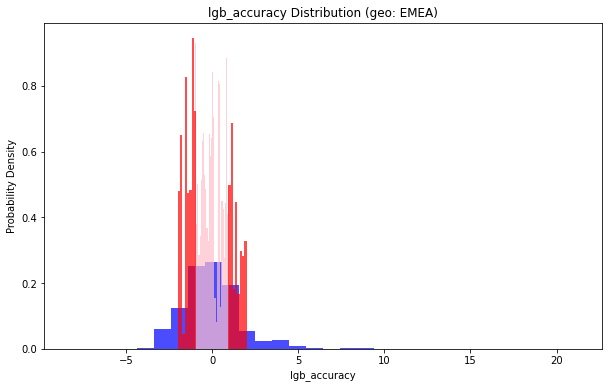
plt.title(f'lgb_accuracy Distribution (geo: {geo})')
plt.xlabel('lgb_accuracy')
plt.ylabel('Probability Density')
ratio_lt_1 = len(lt_pu_pod[np.abs(lt_pu_pod) < 1]) / len(lt_pu_pod)
ratio_lt_2 = len(lt_pu_pod[(np.abs(lt_pu_pod) >= 1) & (np.abs(lt_pu_pod) < 2)]) / len(lt_pu_pod)
print(f'地理位置(geo: {geo})小于1的部分占比:{ratio_lt_1}')
print(f'地理位置(geo: {geo})小于2的部分占比:{ratio_lt_2+ratio_lt_1}')
plt.show()
地理位置(geo: LAS)小于1的部分占比:0.22381331211880137
地理位置(geo: LAS)小于2的部分占比:0.45054362238133117
地理位置(geo: AP)小于1的部分占比:0.45124831309041835
地理位置(geo: AP)小于2的部分占比:0.7465418353576248
地理位置(geo: EMEA)小于1的部分占比:0.5302100017796761
地理位置(geo: EMEA)小于2的部分占比:0.8165153941982559
地理位置(geo: NA)小于1的部分占比:0.39419974342028535
地理位置(geo: NA)小于2的部分占比:0.647980406639972
地理位置(geo: Brazil)小于1的部分占比:0.0
地理位置(geo: Brazil)小于2的部分占比:1.0
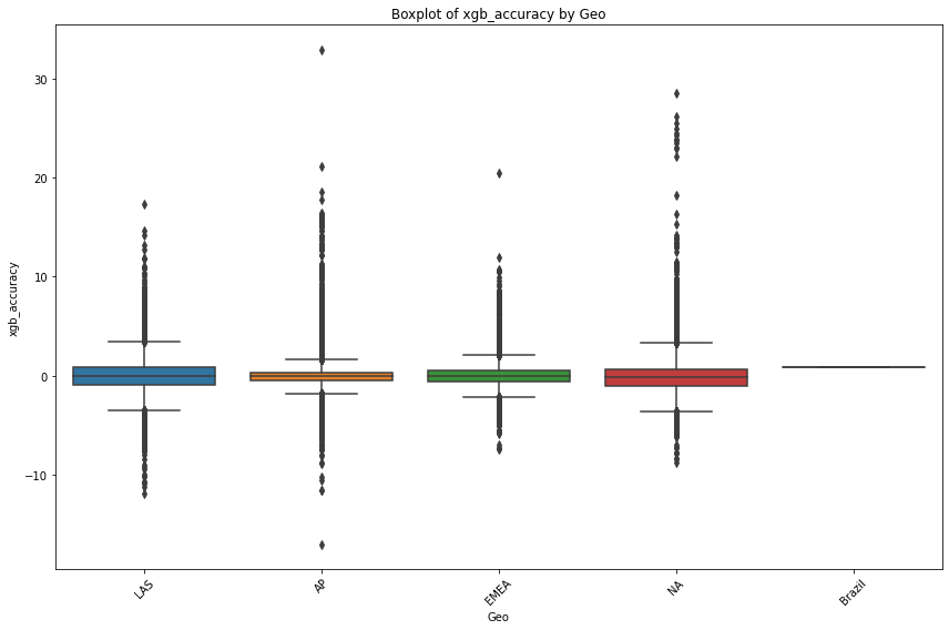
plt.figure(figsize=(12, 8))
sns.boxplot(data=df_replen_2, x='geo', y='xgb_accuracy')
plt.xlabel('Geo')
plt.ylabel('xgb_accuracy')
plt.title('Boxplot of xgb_accuracy by Geo')
plt.xticks(rotation=45)
plt.tight_layout()
plt.show()
group_mot_climate_pu_atd_lgb = df_replen_2.groupby(['geo','mot']).agg({'lgb_accuracy':['std','count','mean',lambda x:x.quantile(0.5),lambda x:x.quantile(0.9),lambda x:x.quantile(0.1)]}).reset_index()
group_mot_climate_pu_atd_lgb.columns = ['geo','mot','std','count','mean','quantile_5','quantile_9','quantile_1']
group_mot_climate_pu_atd_lgb
| geo | mot | std | count | mean | quantile_5 | quantile_9 | quantile_1 |
|---|
| 0 | AP | AIR | 2.342541 | 37683 | -0.040538 | -0.456005 | 2.381934 | -2.108590 |
|---|
| 1 | AP | SEA | 2.965705 | 7366 | 0.021388 | -0.426507 | 3.936324 | -3.207305 |
|---|
| 2 | AP | TRUCK | 0.922056 | 2375 | -0.280426 | -0.378388 | 0.641612 | -1.111371 |
|---|
| 3 | Brazil | AIR | NaN | 1 | 1.869254 | 1.869254 | 1.869254 | 1.869254 |
|---|
group_mot_climate_pu_atd_xgb = df_replen_2.groupby(['geo','mot']).agg({'xgb_accuracy':['std','count','mean',lambda x:x.quantile(0.5),lambda x:x.quantile(0.9),lambda x:x.quantile(0.1)]}).reset_index()
group_mot_climate_pu_atd_xgb.columns = ['geo','mot','std','count','mean','quantile_5','quantile_9','quantile_1']
group_mot_climate_pu_atd_xgb
| geo | mot | std | count | mean | quantile_5 | quantile_9 | quantile_1 |
|---|
| 0 | AP | AIR | 1.578557 | 37683 | 0.003911 | -0.083548 | 1.231544 | -1.290093 |
|---|
| 1 | AP | SEA | 1.442503 | 7366 | -0.001473 | 0.000532 | 1.020673 | -1.118309 |
|---|
| 2 | AP | TRUCK | 0.599171 | 2375 | -0.006152 | -0.085521 | 0.670907 | -0.483689 |
|---|
| 3 | Brazil | AIR | NaN | 1 | 0.874765 | 0.874765 | 0.874765 | 0.874765 |
|---|
| 4 | EMEA | AIR | 1.248103 | 21557 | 0.002630 | -0.047782 | 1.242728 | -1.269656 |
|---|
| 5 | EMEA | SEA | 1.317035 | 919 | 0.073530 | 0.004353 | 0.562636 | -0.495532 |
|---|


 被折叠的 条评论
为什么被折叠?
被折叠的 条评论
为什么被折叠?
 到【灌水乐园】发言


