day21:形状检测

1：直线检测：

根据前面的分析可以得到霍夫变换中存在的两个重要的结论：

(1)图像空间中的每条直线在参 数空间 中都 对应着单一 一个点来表示

(2)图像空间中的直线上任何像素点在参数空间对应的直线 相交 于同一 个点 .

因此通过霍夫变换寻找图像中的直线就 是寻找参数空间中大量直线相交的一点.

但是当图像中存在垂直直 线时，即所有的像素点的x坐标相同时， 直线上的像素点利用上述霍夫变换方法得到的参数空间中 多条直线互相平行，无法相交于一点.

为了解决垂直直线在参数空间没有交点的问题，一般采用极坐标方式表示图像空间 x-y 直角坐标系中的直线，具体形式：

r = xcosθ+ ysinθ    其中r为坐标原点到直线的距离,θ为坐标原点到直线的垂线与X轴的夹角.

根据霍夫变换原理, 利用极坐标形式表示直线时, 在图像空间中经过某一点的所有直线映射到参数空间中是一条正弦曲线。图像空间中直线上的两个点在参数空间中映射的两条正弦曲线相交于一

点，图 给出了用极坐标形式表示直线的霍夫变换的示意图

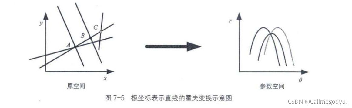
通过上述的变换过程，将图像中的直线检测转换成了在参数空间中寻找某个点 （r,θ）通过的正弦曲线最多的问题. 由于在参数空间内的曲线是连续的 ，而在实际情况中图像的像素是离散的，我们需要将参数空间的θ轴和r轴进行离散化，用离散后的方格表示每一条正弦曲线.首先寻找符合条件的网格，之后寻找该网格对应的图像空间中所有的点，这些点共同组成了原图像中的直线.

总结 上面所有的原理和步骤 ，霍 夫变换算法检测图像中的直线主要分为以下4 个步骤.

第一步 ：将参数空间的坐标轴离散化，例如 θ = 10°，20°，30°.....

                r = 0.1，0.2，0.3....

第二步： 将图像中每个非零像素通过映射关系求取在参数空间通过的方格。

第三步： 统计参数空间内每个方格出现的次数，选取次数大于某一阈值的方格作为表示直线的

              方格.

第四 步 : 将参数空间中表示直线的方格的参数作为图像中直线的参数.

 

 代码：

void drawline(Mat& img, vector<Vec2f> pt,int  width, int  height, Scalar scalar1, int thin)//分别为绘制的图像，直线检测的结果，图像宽，高，颜色，直线宽度
{
	Point p1, p2;//直线上两点
	for (size_t i = 0; i < pt.size(); ++i)
	{
		float r = pt[i][0];//直线检测结果中的r
		float threta = pt[i][1];//直线检测结果中的threta
		double a = cos(threta);//余弦
		double b = sin(threta);//正弦
		double x = a * r;//直线与垂线交点横坐标
		double y = b * r;//直线与垂线交点纵坐标
		double length = max( height,width);
		p1.x = cvRound(x + length * (-b));
		p1.y = cvRound(y + length * (a));
		p2.x = cvRound(x - length * (-b));
		p2.y = cvRound(y - length * (a));
		//cout << p1 << endl;
		//cout << p2 << endl;
		line(img, p1, p2, scalar1, thin);
	}
}
void visionagin::Mylinedetect()
{
	Mat src = imread("C:\\Users\\86176\\Downloads\\visionimage\\build.jfif");
	Mat canny_res;
	Canny(src, canny_res, 80, 180,3,false);//输出边缘检测结果
	threshold(canny_res, canny_res, 170, 255, THRESH_BINARY);//二值化，用于直线检测
	imshow("src", canny_res);
	vector<Vec2f> line1, line2;
	HoughLines(canny_res, line1, 1,CV_PI/180, 250,0,0);//阈值设置过小会无法得到结果
	HoughLines(canny_res, line2, 1, CV_PI / 180, 50,0,0);//line1为直线检测结果，直线极坐标描述的系数，是一个 N * 2 的vector<Vec2f>矩阵，
												//每一行中的第一个元素是直线距离坐标原点的距离R,第二个元素是该直线过坐标原点的垂线与x轴的夹角.
	
	//调用draw函数，将直线检测结果绘出
	Mat res1, res2;
	src.copyTo(res1);
	src.copyTo(res2);
	drawline(res1, line1, canny_res.cols, canny_res.rows, Scalar(255,255,255), 2);
	drawline(res2, line1, canny_res.cols, canny_res.rows, Scalar(0,0,255), 1);
	imshow("res1", res1);
	imshow("res2", res2);

}

结果：

 

 代码：

void visionagin::Mylinedetect2()
{
	Mat src = imread("C:\\Users\\86176\\Downloads\\visionimage\\build.jfif");
	imshow("原图", src);
	Mat canny_res;
	Canny(src, canny_res, 220, 240, 3, false);
	threshold(canny_res, canny_res, 180, 255, THRESH_BINARY);
	imshow("cannyres", canny_res);
	vector<Vec4f>line1;
	HoughLinesP(canny_res, line1,1,CV_PI/180,200,150,20);
	Mat img;
	src.copyTo(img);
	for (int i = 0; i < line1.size(); ++i)
	{
		line(img, Point(line1[i][0], line1[i][1]), Point(line1[i][2], line1[i][3]), Scalar(0, 0, 200), 1);
	}
	imshow("houghlinep", img);
}

代码：

void visionagin:: Mylinedetect3()
{
	float Point[15][2] = {
		{0.0f, 369.0 }, {10.0, 364.0},{ 20.0,358.0 }, { 30.0f,352.0 },{ 40.0, 346.0 }, { 50.0, 341.0}, {60.0,335.0}, { 70.0,329.0 },
		{ 50.0, 316.0 }, { 30, 311.0}, {30,335.0}, { 70.0,339.0 },{4.0f, 349.0 }, {15.0, 344.0},{ 20.0,328.0 }
	};
	vector<Point2f>Points;
	for(int i = 0; i < 15; ++i)
	{
		Points.push_back(Point2f(Point[i][0], Point[i][1]));
	}
	Mat lines;
	int linesmax = 20;
	int linesthreshold = 1;
	double minrho = 0;//最小长度
	double maxrho = 360;//最大长度
	double rhostep = 1;//离散化单位长度
	double mintheta = 0;//最小角度
	double maxthtea = CV_PI / 2;//最大 角度
	double thetastep = CV_PI / 180;//离散化单位角度
	HoughLinesPointSet(Points, lines, 20, 1,minrho, maxrho, rhostep, mintheta, maxthtea, thetastep);
	vector<Vec3d> lines3d;
	lines.copyTo(lines3d);
	for (int j = 0; j < lines3d.size(); ++j)
	{
		cout << "votes:" << lines3d.at(j).val[0] ;
		cout << " r: " << lines3d.at(j).val[1] ;
		cout << " threta: " << lines3d.at(j).val[2] << endl;
	}
}

 2：直线拟合：

void visionagin::Myfitline()
{
	double Point[10][2] = {
		{1.1,1.0},{2,2.1},{2.9,3.1},{4.2,4.0},{5,5.1},
		{6.1,5.9},{7.1,6.8},{8,8.1},{9.0,9.1},{10,10.1}
	};//含有误差的点集
	Vec4f line;
	vector<Point2f> Points;
	for (int i = 0; i < 10; ++i)
	{
		Points.push_back(Point2f(Point[i][0], Point[i][1]));
	}
	fitLine(Points, line, DIST_L1, 0, 0.01, 0.01);
	cout << " k= " << line[2] / line[3] << endl;
	cout << "直线上一点，x= " << line[2] << " , y= " << line[3];
	cout << "该直线为：y= " << line[2] / line[3] << "(x-" << line[2] << ")+" << line[3];
}

3：圆形检测：

实现：

void  visionagin::Mycircledetect()
{
	Mat src = imread("C:\\Users\\86176\\Downloads\\visionimage\\coin.jfif");
	Mat gauss;
	GaussianBlur(src, gauss, Size(3, 3),2,2);
	imshow("gauss", gauss);
	Mat gry;
	cvtColor(gauss, gry, COLOR_BGR2GRAY);
	vector<Vec3f> circles;
	double dp = 2;//分辨率变为一半
	double mindist = 10;//圆心间最小距离
	double parpm1 = 400;//canny阈值中的较大值
	double parpm2 = 90;//检测圆形的累加器阙值 值越大 检测的圆形越精确.
	int minr = 0;
	int maxr = 100;
	HoughCircles(gry, circles, HOUGH_GRADIENT, dp, mindist, parpm1, parpm2,minr,maxr);
	Mat res;
	src.copyTo(res);
	for (size_t i = 0; i < circles.size(); ++i)
	{
		Point2f center;
		center.x =cvRound( circles[i][0]);
		center.y =cvRound( circles[i][1]);
		double r = circles[i][2];
		circle(res, center, 2, Scalar(0, 0,255), -1);
		circle(res, center, r, Scalar(0, 0, 200), 2);
	}
	imshow("src", src);
	imshow("res", res);
}