Logistic逻辑回归算法学习（一）

目录

一、什么是逻辑回归

二、逻辑回顾的损失函数

三、实现逻辑回归算法

1、自定义一个LogisticRegression 类

2、测试

---

一、什么是逻辑回归

---

逻辑回归主要解决分类问题，通常只可以解决二分类问题。实际上逻辑回归的原理是将样本的特征和样本发生的概率联系起来，由于概率是一个数，因此也可以叫做一个回归算法。

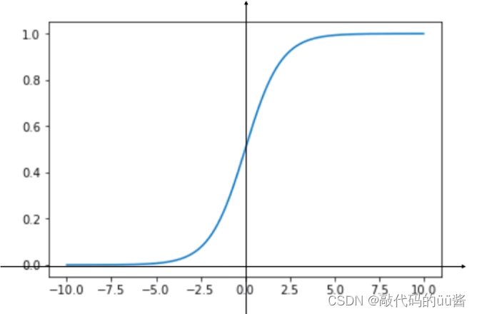
在这里，引入一个函数Sigmoid，它的公式如下：

值域为(0,1)

• 当 t > 0 时，p > 0.5
• 当 t < 0 时，p < 0.5

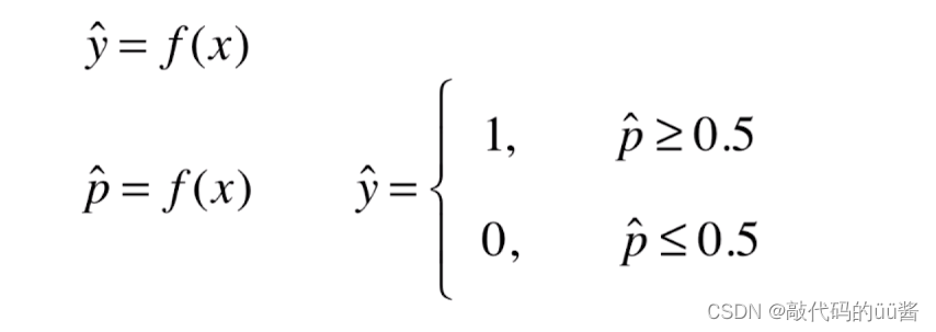
因此，概率估计值求解公式转换为       

基于此，对于给定的样本数据集X,y，我们如何找到参数theta，使得用这样的方式可以最大程度获得样本数据集X对应的分类输出y？

二、逻辑回顾的损失函数

---

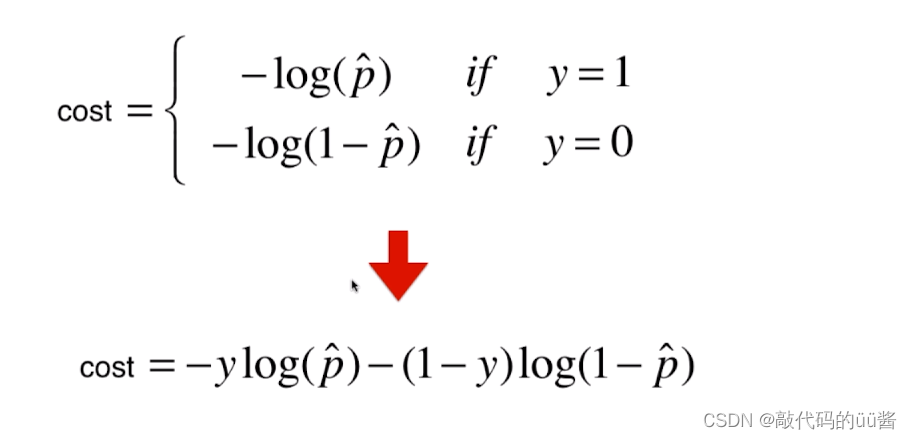
根据该公式定义一个损失函数，如果给定一个样本，当

• y = 1，p越小，cost越大
• y = 0，p越大，cost越大

基于此，对于逻辑回归，m个样本的损失函数可以定义为：

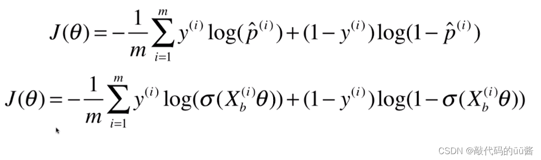
该损失函数没有公式解，只能使用梯度下降法求解。

三、实现逻辑回归算法

---

1、自定义一个LogisticRegression 类

代码示例：

import numpy as np
from sklearn.metrics import accuracy_score

class LogisticRegression:
    def __int__(self):
        ''' 初始化Logistic Regression模型'''
        self.coef_ = None
        self.interception_ = None
        self._theta = None

    def _sigmoid(self,t):
        return 1. / (1. + np.exp(-t))

    def fit(self,X_train,y_train,eta=0.01,n_iters=1e4):
        '''  根据训练数据集X_train,y_train，使用梯度下降法训练Logistic Regression模型'''
        assert X_train.shape[0] == y_train.shape[0], \
            "the size of X_train must be equal to the size of y_train"

        # 逻辑回顾损失函数实现
        def J(theta, X_b, y):
            y_hat = self._sigmoid(X_b.dot(theta))
            try:
                return - np.sum(y*np.log(y_hat) + (1-y)*np.log(1-y_hat)) / len(y)
            except:
                return float('inf')

        # 逻辑回归求梯度
        def dJ(theta, x_b, y):
            return x_b.T.dot(self._sigmoid(x_b.dot(theta)) - y) / len(x_b)

        def gradient_descent(x_b, y, initial_theta, eta, n_iters=1e4, epsilon=1e-8):

            theta = initial_theta
            i_iter = 0

            while i_iter < n_iters:
                gradient = dJ(theta, x_b, y)
                last_theta = theta
                theta = theta - eta * gradient

                if (abs(J(theta, x_b, y) - J(last_theta, x_b, y)) < epsilon):
                    break

                i_iter += 1

            return theta

        x_b = np.hstack([np.ones((len(X_train), 1)), X_train])
        initial_theta = np.zeros(x_b.shape[1])
        self._theta = gradient_descent(x_b,y_train,initial_theta,eta,n_iters)

        self.interception_ = self._theta[0]  # 截距
        self.coef_ = self._theta[1:]  # 斜率

        return self

    def predict_proba(self,X_predict):
        """ 给定待预测数据集X_predicr,返回表示X_predict的结果概率向量"""
        assert self.interception_ is not None and self.coef_ is not None, \
            "must fit before predict!"

        assert X_predict.shape[1] == len(self.coef_), \
            "the feature number of X_predict must be equal to X_train"

        X_b = np.hstack([np.ones((len(X_predict), 1)), X_predict])
        return self._sigmoid(X_b.dot(self._theta))
    def predict(self,X_predict):
        """ 给定待预测数据集X_predicr,返回表示X_predict的结果向量"""
        assert self.interception_ is not None and self.coef_ is not None, \
            "must fit before predict!"

        assert X_predict.shape[1] == len(self.coef_), \
            "the feature number of X_predict must be equal to X_train"

        proba = self.predict_proba(X_predict)  #概率
        return np.array(proba >= 0.5,dtype='int')  #强制将返回的布尔转换成数值0和1，代表两个不同的类别

    def score(self,X_test,y_test):
        """ 根据测试数据集 X_test 和 y_test 确定当前模型的准确度 """
        y_predict = self.predict(X_test)
        return accuracy_score(y_test,y_predict)

    def __repr__(self):
        return "LogisticRegression()"

2、测试

代码示例：

import numpy as np
import matplotlib.pyplot as plt
from sklearn import datasets

iris = datasets.load_iris()
X = iris.data
y = iris.target

X = X[y<2, :2]  #对于X的每一行选取y=0和y=1的行
y = y[y<2]

from sklearn.model_selection import train_test_split

X_train,X_test,y_train,y_test = train_test_split(X,y,random_state = 666)


from mySklearn.LogisticRegression import LogisticRegression
log_reg = LogisticRegression()
log_reg.fit(X_train,y_train)

log_reg.score(X_test,y_test)
log_reg.predict_proba(X_test)

运行结果：

数组中的每一个元素都有相应的一个概率值，概率值越趋近于1，模型就更愿意将这个样本分类为1，越趋近于0，则将样本分类为0。