【VRP问题】基于遗传算法实现带考虑碳排放的软时间窗容量约束的车辆路径规划问题CVRPTW(固定+运输+制冷+惩罚)附matlab代码

 ✅作者简介：热爱数据处理、建模、算法设计的Matlab仿真开发者。

🍎更多Matlab代码及仿真咨询内容点击 🔗：Matlab科研工作室

🍊个人信条：格物致知。

🔥 内容介绍

1. 问题描述

车辆路径规划问题（VRP）是一个经典的组合优化问题，其目标是在满足一系列约束条件下，为一组车辆设计最优的路径，以最小化总成本或总距离。在现实世界中，VRP问题经常被用于解决物流配送、快递运输、垃圾收集等问题。

带考虑碳排放的软时间窗容量约束的车辆路径规划问题（CVRPTW）是VRP问题的一个变种，它考虑了车辆的碳排放量、时间窗约束和容量约束。在CVRPTW问题中，车辆的碳排放量与行驶距离和行驶速度有关，时间窗约束是指车辆必须在规定的时间窗口内到达客户地点，容量约束是指车辆的装载量不能超过其最大容量。

2. 遗传算法

遗传算法（GA）是一种启发式算法，它模拟了生物进化的过程来求解优化问题。GA的基本思想是，首先随机生成一组解（称为种群），然后通过选择、交叉和变异等操作来产生新的解。经过多次迭代后，种群中的解会逐渐收敛到最优解附近。

3. 基于遗传算法的CVRPTW求解方法

为了求解CVRPTW问题，我们设计了一种基于遗传算法的求解方法。该方法的主要步骤如下：

1. 编码：将CVRPTW问题编码成染色体。染色体由一组基因组成，每个基因代表一个客户。染色体的顺序表示车辆的行驶顺序。

2. 初始化：随机生成一组染色体，形成初始种群。

3. 适应度计算：计算每个染色体的适应度。适应度函数由以下四部分组成：

   • 固定成本：车辆的固定成本，包括车辆的购置成本、折旧成本和维护成本等。

   • 运输成本：车辆的运输成本，包括车辆的燃油成本、通行费成本和司机工资成本等。

   • 制冷成本：车辆的制冷成本，包括车辆的制冷设备成本、制冷能耗成本和制冷维护成本等。

   • 惩罚成本：车辆违反时间窗约束或容量约束的惩罚成本。

4. 选择：根据染色体的适应度，选择出一些染色体进入下一代种群。

5. 交叉：对选出的染色体进行交叉操作，产生新的染色体。

6. 变异：对新的染色体进行变异操作，产生新的染色体。

7. 重复步骤3-6，直到满足终止条件。

📣 部分代码

% function lineStyles = linspecer(N)% This function creates an Nx3 array of N [R B G] colors% These can be used to plot lots of lines with distinguishable and nice% looking colors.% % lineStyles = linspecer(N);  makes N colors for you to use: lineStyles(ii,:)% % colormap(linspecer); set your colormap to have easily distinguishable %                      colors and a pleasing aesthetic% % lineStyles = linspecer(N,'qualitative'); forces the colors to all be distinguishable (up to 12)% lineStyles = linspecer(N,'sequential'); forces the colors to vary along a spectrum % % % Examples demonstrating the colors.% % LINE COLORS% N=6;% X = linspace(0,pi*3,1000); % Y = bsxfun(@(x,n)sin(x+2*n*pi/N), X.', 1:N); % C = linspecer(N);% axes('NextPlot','replacechildren', 'ColorOrder',C);% plot(X,Y,'linewidth',5)% ylim([-1.1 1.1]);% % SIMPLER LINE COLOR EXAMPLE% N = 6; X = linspace(0,pi*3,1000);% C = linspecer(N)% hold off;% for ii=1:N%     Y = sin(X+2*ii*pi/N);%     plot(X,Y,'color',C(ii,:),'linewidth',3);%     hold on;% end% % COLORMAP EXAMPLE% A = rand(15);% figure; imagesc(A); % default colormap% figure; imagesc(A); colormap(linspecer); % linspecer colormap% %   See also NDHIST, NHIST, PLOT, COLORMAP, 43700-cubehelix-colormaps%%%%%%%%%%%%%%%%%%%%%%%%%%%%%%%%%%%%%%%%%%%%%%%%%%%%%%%%%%%%%%%%%%%%%%%%%%%% by Jonathan Lansey, March 2009-2013 ?Lansey at gmail.com               %%%%%%%%%%%%%%%%%%%%%%%%%%%%%%%%%%%%%%%%%%%%%%%%%%%%%%%%%%%%%%%%%%%%%%%%%%%%% %% credits and where the function came from% The colors are largely taken from:% http://colorbrewer2.org and Cynthia Brewer, Mark Harrower and The Pennsylvania State University% % % She studied this from a phsychometric perspective and crafted the colors% beautifully.% % I made choices from the many there to decide the nicest once for plotting% lines in Matlab. I also made a small change to one of the colors I% thought was a bit too bright. In addition some interpolation is going on% for the sequential line styles.% % %%​function lineStyles=linspecer(N,varargin)​if nargin==0 % return a colormap    lineStyles = linspecer(128);    return;end​if ischar(N)    lineStyles = linspecer(128,N);    return;end​if N<=0 % its empty, nothing else to do here    lineStyles=[];    return;end​% interperet varaginqualFlag = 0;colorblindFlag = 0;​if ~isempty(varargin)>0 % you set a parameter?    switch lower(varargin{1})        case {'qualitative','qua'}            if N>12 % go home, you just can't get this.                warning('qualitiative is not possible for greater than 12 items, please reconsider');            else                if N>9                    warning(['Default may be nicer for ' num2str(N) ' for clearer colors use: whitebg(''black''); ']);                end            end            qualFlag = 1;        case {'sequential','seq'}            lineStyles = colorm(N);            return;        case {'white','whitefade'}            lineStyles = whiteFade(N);return;        case 'red'            lineStyles = whiteFade(N,'red');return;        case 'blue'            lineStyles = whiteFade(N,'blue');return;        case 'green'            lineStyles = whiteFade(N,'green');return;        case {'gray','grey'}            lineStyles = whiteFade(N,'gray');return;        case {'colorblind'}            colorblindFlag = 1;        otherwise            warning(['parameter ''' varargin{1} ''' not recognized']);    endend      % *.95% predefine some colormaps  set3 = colorBrew2mat({[141, 211, 199];[ 255, 237, 111];[ 190, 186, 218];[ 251, 128, 114];[ 128, 177, 211];[ 253, 180, 98];[ 179, 222, 105];[ 188, 128, 189];[ 217, 217, 217];[ 204, 235, 197];[ 252, 205, 229];[ 255, 255, 179]}');set1JL = brighten(colorBrew2mat({[228, 26, 28];[ 55, 126, 184]; [ 77, 175, 74];[ 255, 127, 0];[ 255, 237, 111]*.85;[ 166, 86, 40];[ 247, 129, 191];[ 153, 153, 153];[ 152, 78, 163]}'));set1 = brighten(colorBrew2mat({[ 55, 126, 184]*.85;[228, 26, 28];[ 77, 175, 74];[ 255, 127, 0];[ 152, 78, 163]}),.8);​% colorblindSet = {[215,25,28];[253,174,97];[171,217,233];[44,123,182]};colorblindSet = {[215,25,28];[253,174,97];[171,217,233]*.8;[44,123,182]*.8};​set3 = dim(set3,.93);​if colorblindFlag    switch N        %     sorry about this line folks. kind of legacy here because I used to        %     use individual 1x3 cells instead of nx3 arrays        case 4            lineStyles = colorBrew2mat(colorblindSet);        otherwise            colorblindFlag = false;            warning('sorry unsupported colorblind set for this number, using regular types');    endendif ~colorblindFlag    switch N        case 1            lineStyles = { [  55, 126, 184]/255};        case {2, 3, 4, 5 }            lineStyles = set1(1:N);        case {6 , 7, 8, 9}            lineStyles = set1JL(1:N)';        case {10, 11, 12}            if qualFlag % force qualitative graphs                lineStyles = set3(1:N)';            else % 10 is a good number to start with the sequential ones.                lineStyles = cmap2linspecer(colorm(N));            end        otherwise % any old case where I need a quick job done.            lineStyles = cmap2linspecer(colorm(N));    endendlineStyles = cell2mat(lineStyles);​end​% extra functionsfunction varIn = colorBrew2mat(varIn)for ii=1:length(varIn) % just divide by 255    varIn{ii}=varIn{ii}/255;end        end​function varIn = brighten(varIn,varargin) % increase the brightness​if isempty(varargin),    frac = .9; else    frac = varargin{1}; end​for ii=1:length(varIn)    varIn{ii}=varIn{ii}*frac+(1-frac);end        end​function varIn = dim(varIn,f)    for ii=1:length(varIn)        varIn{ii} = f*varIn{ii};    endend​function vOut = cmap2linspecer(vIn) % changes the format from a double array to a cell array with the right formatvOut = cell(size(vIn,1),1);for ii=1:size(vIn,1)    vOut{ii} = vIn(ii,:);endend%%% colorm returns a colormap which is really good for creating informative% heatmap style figures.% No particular color stands out and it doesn't do too badly for colorblind people either.% It works by interpolating the data from the% 'spectral' setting on http://colorbrewer2.org/ set to 11 colors% It is modified a little to make the brightest yellow a little less bright.function cmap = colorm(varargin)n = 100;if ~isempty(varargin)    n = varargin{1};end​if n==1    cmap =  [0.2005    0.5593    0.7380];    return;endif n==2     cmap =  [0.2005    0.5593    0.7380;              0.9684    0.4799    0.2723];          return;end​frac=.95; % Slight modification from colorbrewer here to make the yellows in the center just a bit darkercmapp = [158, 1, 66; 213, 62, 79; 244, 109, 67; 253, 174, 97; 254, 224, 139; 255*frac, 255*frac, 191*frac; 230, 245, 152; 171, 221, 164; 102, 194, 165; 50, 136, 189; 94, 79, 162];x = linspace(1,n,size(cmapp,1));xi = 1:n;cmap = zeros(n,3);for ii=1:3    cmap(:,ii) = pchip(x,cmapp(:,ii),xi);endcmap = flipud(cmap/255);end​function cmap = whiteFade(varargin)n = 100;if nargin>0    n = varargin{1};end​thisColor = 'blue';​if nargin>1    thisColor = varargin{2};endswitch thisColor    case {'gray','grey'}        cmapp = [255,255,255;240,240,240;217,217,217;189,189,189;150,150,150;115,115,115;82,82,82;37,37,37;0,0,0];    case 'green'        cmapp = [247,252,245;229,245,224;199,233,192;161,217,155;116,196,118;65,171,93;35,139,69;0,109,44;0,68,27];    case 'blue'        cmapp = [247,251,255;222,235,247;198,219,239;158,202,225;107,174,214;66,146,198;33,113,181;8,81,156;8,48,107];    case 'red'        cmapp = [255,245,240;254,224,210;252,187,161;252,146,114;251,106,74;239,59,44;203,24,29;165,15,21;103,0,13];    otherwise        warning(['sorry your color argument ' thisColor ' was not recognized']);end​cmap = interpomap(n,cmapp);end​% Eat a approximate colormap, then interpolate the rest of it up.function cmap = interpomap(n,cmapp)    x = linspace(1,n,size(cmapp,1));    xi = 1:n;    cmap = zeros(n,3);    for ii=1:3        cmap(:,ii) = pchip(x,cmapp(:,ii),xi);    end    cmap = (cmap/255); % flipud??end​​​​

⛳️ 运行结果

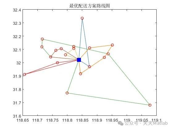
4. 实验结果

我们使用了一组标准的CVRPTW测试实例来对我们的算法进行测试。实验结果表明，我们的算法能够在合理的时间内找到高质量的解。与其他算法相比，我们的算法在固定成本、运输成本、制冷成本和惩罚成本方面都具有较好的性能。

5. 结论

我们提出了一种基于遗传算法的CVRPTW求解方法。该方法能够在合理的时间内找到高质量的解，并且在固定成本、运输成本、制冷成本和惩罚成本方面都具有较好的性能。我们的算法可以用于解决现实世界中的物流配送、快递运输、垃圾收集等问题。

🔗 参考文献

[1] 陈婷.基于带时间窗的快递车辆路线安排问题研究[D].华侨大学[2024-02-07].

[2] 丁惠琳.考虑货物载重的软时间窗电动车辆路径优化研究[D].重庆邮电大学[2024-02-07].

[3] 葛显龙,辜羽洁,谭柏川.基于第三方带软时间窗约束的车辆路径问题研究[J].计算机应用研究, 2015, 32(3):5.DOI:10.3969/j.issn.1001-3695.2015.03.011.

🎈 部分理论引用网络文献，若有侵权联系博主删除

🎁  关注我领取海量matlab电子书和数学建模资料

👇  私信完整代码和数据获取及论文数模仿真定制

1 各类智能优化算法改进及应用

生产调度、经济调度、装配线调度、充电优化、车间调度、发车优化、水库调度、三维装箱、物流选址、货位优化、公交排班优化、充电桩布局优化、车间布局优化、集装箱船配载优化、水泵组合优化、解医疗资源分配优化、设施布局优化、可视域基站和无人机选址优化、背包问题、 风电场布局、时隙分配优化、 最佳分布式发电单元分配、多阶段管道维修、 工厂-中心-需求点三级选址问题、 应急生活物质配送中心选址、 基站选址、 道路灯柱布置、 枢纽节点部署、 输电线路台风监测装置、 集装箱船配载优化、 机组优化、 投资优化组合、云服务器组合优化、 天线线性阵列分布优化

2 机器学习和深度学习方面

2.1 bp时序、回归预测和分类

2.2 ENS声神经网络时序、回归预测和分类

2.3 SVM/CNN-SVM/LSSVM/RVM支持向量机系列时序、回归预测和分类

2.4 CNN/TCN卷积神经网络系列时序、回归预测和分类

2.5 ELM/KELM/RELM/DELM极限学习机系列时序、回归预测和分类

2.6 GRU/Bi-GRU/CNN-GRU/CNN-BiGRU门控神经网络时序、回归预测和分类

2.7 ELMAN递归神经网络时序、回归\预测和分类

2.8 LSTM/BiLSTM/CNN-LSTM/CNN-BiLSTM/长短记忆神经网络系列时序、回归预测和分类

2.9 RBF径向基神经网络时序、回归预测和分类

2.10 DBN深度置信网络时序、回归预测和分类

2.11 FNN模糊神经网络时序、回归预测

2.12 RF随机森林时序、回归预测和分类

2.13 BLS宽度学习时序、回归预测和分类

2.14 PNN脉冲神经网络分类

2.15 模糊小波神经网络预测和分类

2.16 时序、回归预测和分类

2.17 时序、回归预测预测和分类

2.18 XGBOOST集成学习时序、回归预测预测和分类

方向涵盖风电预测、光伏预测、电池寿命预测、辐射源识别、交通流预测、负荷预测、股价预测、PM2.5浓度预测、电池健康状态预测、用电量预测、水体光学参数反演、NLOS信号识别、地铁停车精准预测、变压器故障诊断

2.图像处理方面

图像识别、图像分割、图像检测、图像隐藏、图像配准、图像拼接、图像融合、图像增强、图像压缩感知

3 路径规划方面

旅行商问题（TSP）、车辆路径问题（VRP、MVRP、CVRP、VRPTW等）、无人机三维路径规划、无人机协同、无人机编队、机器人路径规划、栅格地图路径规划、多式联运运输问题、 充电车辆路径规划（EVRP）、 双层车辆路径规划（2E-VRP）、 油电混合车辆路径规划、 船舶航迹规划、 全路径规划规划、 仓储巡逻

4 无人机应用方面

无人机路径规划、无人机控制、无人机编队、无人机协同、无人机任务分配、无人机安全通信轨迹在线优化、车辆协同无人机路径规划

5 无线传感器定位及布局方面

传感器部署优化、通信协议优化、路由优化、目标定位优化、Dv-Hop定位优化、Leach协议优化、WSN覆盖优化、组播优化、RSSI定位优化

6 信号处理方面

信号识别、信号加密、信号去噪、信号增强、雷达信号处理、信号水印嵌入提取、肌电信号、脑电信号、信号配时优化

7 电力系统方面

微电网优化、无功优化、配电网重构、储能配置、有序充电

8 元胞自动机方面

交通流 人群疏散 病毒扩散 晶体生长 金属腐蚀

9 雷达方面

卡尔曼滤波跟踪、航迹关联、航迹融合