


写在前面的一些内容
本次习题来源于 NNDL 作业8:RNN - 简单循环网络 。
水平有限,难免有误,如有错漏之处敬请指正。
习题1
使用Numpy实现简单循环网络.
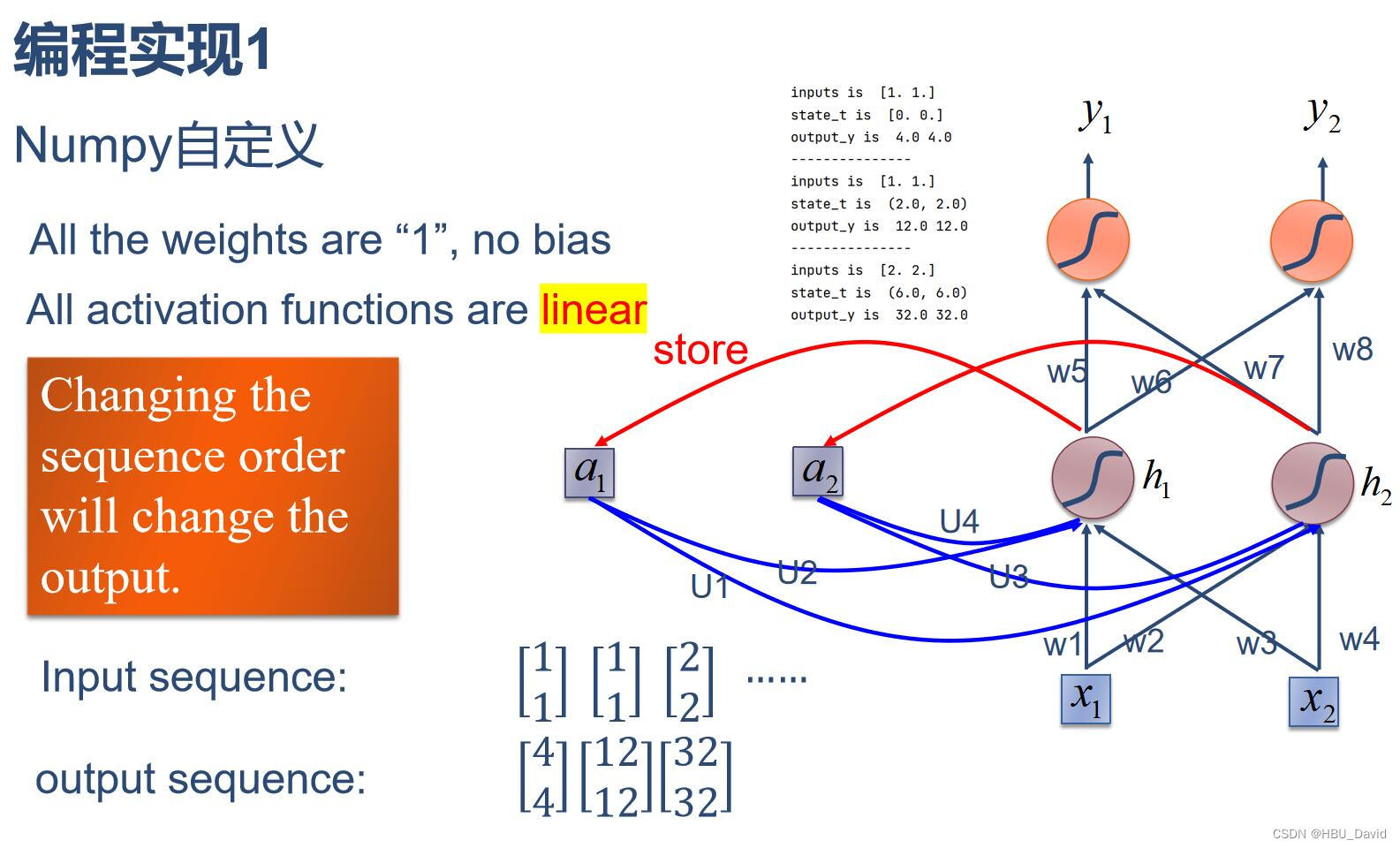
import numpy as np

inputs = np.array([[1., 1.],
                   [1., 1.],
                   [2., 2.]])  # 初始化输入序列
print('inputs is ', inputs)

state_t = np.zeros(2, )  # 初始化存储器
print('state_t is ', state_t)

w1, w2, w3, w4, w5, w6, w7, w8 = 1., 1., 1., 1., 1., 1., 1., 1.
U1, U2, U3, U4 = 1., 1., 1., 1.
print('--------------------------------------')
for input_t in inputs:
    print('inputs is ', input_t)
    print('state_t is ', state_t)
    in_h1 = np.dot([w1, w3], input_t) + np.dot([U2, U4], state_t)
    in_h2 = np.dot([w2, w4], input_t) + np.dot([U1, U3], state_t)
    state_t = in_h1, in_h2
    output_y1 = np.dot([w5, w7], [in_h1, in_h2])
    output_y2 = np.dot([w6, w8], [in_h1, in_h2])
    print('output_y is ', output_y1, output_y2)
    print('---------------')
代码执行结果:
inputs is  [[1. 1.]
 [1. 1.]
 [2. 2.]]
state_t is  [0. 0.]
--------------------------------------
inputs is  [1. 1.]
state_t is  [0. 0.]
output_y is  4.0 4.0
---------------
inputs is  [1. 1.]
state_t is  (2.0, 2.0)
output_y is  12.0 12.0
---------------
inputs is  [2. 2.]
state_t is  (6.0, 6.0)
output_y is  32.0 32.0
---------------
习题2
在习题1的基础上,增加激活函数tanh.

import numpy as np

inputs = np.array([[1., 1.],
                   [1., 1.],
                   [2., 2.]])  # 初始化输入序列
print('inputs is ', inputs)

state_t = np.zeros(2, )  # 初始化存储器
print('state_t is ', state_t)

w1, w2, w3, w4, w5, w6, w7, w8 = 1., 1., 1., 1., 1., 1., 1., 1.
U1, U2, U3, U4 = 1., 1., 1., 1.
print('--------------------------------------')
for input_t in inputs:
    print('inputs is ', input_t)
    print('state_t is ', state_t)
    in_h1 = np.tanh(np.dot([w1, w3], input_t) + np.dot([U2, U4], state_t))
    in_h2 = np.tanh(np.dot([w2, w4], input_t) + np.dot([U1, U3], state_t))
    state_t = in_h1, in_h2
    output_y1 = np.dot([w5, w7], [in_h1, in_h2])
    output_y2 = np.dot([w6, w8], [in_h1, in_h2])
    print('output_y is ', output_y1, output_y2)
    print('---------------')
代码执行结果:
inputs is  [[1. 1.]
 [1. 1.]
 [2. 2.]]
state_t is  [0. 0.]
--------------------------------------
inputs is  [1. 1.]
state_t is  [0. 0.]
output_y is  1.9280551601516338 1.9280551601516338
---------------
inputs is  [1. 1.]
state_t is  (0.9640275800758169, 0.9640275800758169)
output_y is  1.9984510891336251 1.9984510891336251
---------------
inputs is  [2. 2.]
state_t is  (0.9992255445668126, 0.9992255445668126)
output_y is  1.9999753470497836 1.9999753470497836
---------------
习题3
分别使用nn.RNNCell、nn.RNN实现简单循环网络.
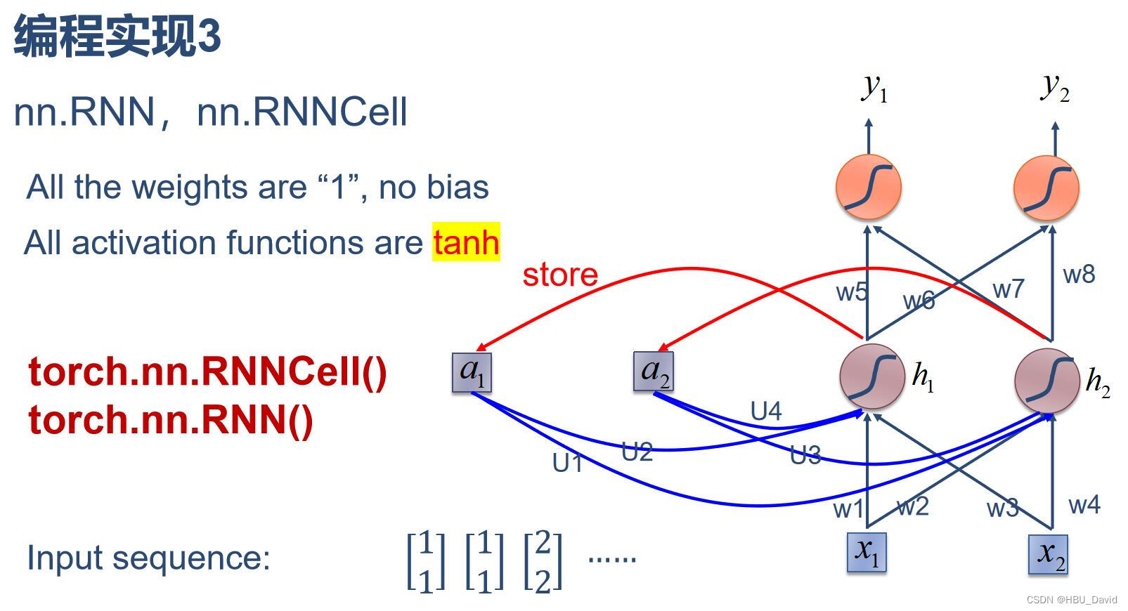
nn.RNNCell实现
RNNCell是TensorFlow中实现RNN的基本单元。
import torch

batch_size = 1
seq_len = 3  # 序列长度
input_size = 2  # 输入序列维度
hidden_size = 2  # 隐藏层维度
output_size = 2  # 输出层维度

# RNNCell
cell = torch.nn.RNNCell(input_size=input_size, hidden_size=hidden_size)
# 初始化参数 https://zhuanlan.zhihu.com/p/342012463
for name, param in cell.named_parameters():
    if name.startswith("weight"):
        torch.nn.init.ones_(param)
    else:
        torch.nn.init.zeros_(param)
# 线性层
liner = torch.nn.Linear(hidden_size, output_size)
liner.weight.data = torch.Tensor([[1, 1], [1, 1]])
liner.bias.data = torch.Tensor([0.0])

seq = torch.Tensor([[[1, 1]],
                    [[1, 1]],
                    [[2, 2]]])
hidden = torch.zeros(batch_size, hidden_size)
output = torch.zeros(batch_size, output_size)

for idx, input in enumerate(seq):
    print('=' * 20, idx, '=' * 20)

    print('Input :', input)
    print('hidden :', hidden)

    hidden = cell(input, hidden)
    output = liner(hidden)
    print('output :', output)
代码执行结果:
==================== 0 ====================
Input : tensor([[1., 1.]])
hidden : tensor([[0., 0.]])
output : tensor([[1.9281, 1.9281]], grad_fn=<AddmmBackward0>)
==================== 1 ====================
Input : tensor([[1., 1.]])
hidden : tensor([[0.9640, 0.9640]], grad_fn=<TanhBackward0>)
output : tensor([[1.9985, 1.9985]], grad_fn=<AddmmBackward0>)
==================== 2 ====================
Input : tensor([[2., 2.]])
hidden : tensor([[0.9992, 0.9992]], grad_fn=<TanhBackward0>)
output : tensor([[2.0000, 2.0000]], grad_fn=<AddmmBackward0>)
nn.RNN实现
import torch

batch_size = 1
seq_len = 3
input_size = 2
hidden_size = 2
num_layers = 1
output_size = 2

cell = torch.nn.RNN(input_size=input_size, hidden_size=hidden_size, num_layers=num_layers)
for name, param in cell.named_parameters():  # 初始化参数
    if name.startswith("weight"):
        torch.nn.init.ones_(param)
    else:
        torch.nn.init.zeros_(param)

# 线性层
liner = torch.nn.Linear(hidden_size, output_size)
liner.weight.data = torch.Tensor([[1, 1], [1, 1]])
liner.bias.data = torch.Tensor([0.0])

inputs = torch.Tensor([[[1, 1]],
                       [[1, 1]],
                       [[2, 2]]])
hidden = torch.zeros(num_layers, batch_size, hidden_size)
out, hidden = cell(inputs, hidden)

print('Input :', inputs[0])
print('hidden:', 0, 0)
print('Output:', liner(out[0]))
print('--------------------------------------')
print('Input :', inputs[1])
print('hidden:', out[0])
print('Output:', liner(out[1]))
print('--------------------------------------')
print('Input :', inputs[2])
print('hidden:', out[1])
print('Output:', liner(out[2]))
代码执行结果:
Input : tensor([[1., 1.]])
hidden: 0 0
Output: tensor([[1.9281, 1.9281]], grad_fn=<AddmmBackward0>)
--------------------------------------
Input : tensor([[1., 1.]])
hidden: tensor([[0.9640, 0.9640]], grad_fn=<SelectBackward0>)
Output: tensor([[1.9985, 1.9985]], grad_fn=<AddmmBackward0>)
--------------------------------------
Input : tensor([[2., 2.]])
hidden: tensor([[0.9992, 0.9992]], grad_fn=<SelectBackward0>)
Output: tensor([[2.0000, 2.0000]], grad_fn=<AddmmBackward0>)
习题4
分析“二进制加法” 源代码。
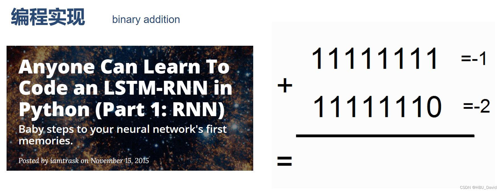
import copy, numpy as np

np.random.seed(0)


# compute sigmoid nonlinearity
def sigmoid(x):
    output = 1 / (1 + np.exp(-x))
    return output


# convert output of sigmoid function to its derivative
def sigmoid_output_to_derivative(output):
    return output * (1 - output)


# training dataset generation
int2binary = {}
binary_dim = 8

largest_number = pow(2, binary_dim)
binary = np.unpackbits(
    np.array([range(largest_number)], dtype=np.uint8).T, axis=1)
for i in range(largest_number):
    int2binary[i] = binary[i]

# input variables
alpha = 0.1
input_dim = 2
hidden_dim = 16
output_dim = 1

# initialize neural network weights
synapse_0 = 2 * np.random.random((input_dim, hidden_dim)) - 1
synapse_1 = 2 * np.random.random((hidden_dim, output_dim)) - 1
synapse_h = 2 * np.random.random((hidden_dim, hidden_dim)) - 1

synapse_0_update = np.zeros_like(synapse_0)
synapse_1_update = np.zeros_like(synapse_1)
synapse_h_update = np.zeros_like(synapse_h)

# training logic
for j in range(10000):

    # generate a simple addition problem (a + b = c)
    a_int = np.random.randint(largest_number / 2)  # int version
    a = int2binary[a_int]  # binary encoding

    b_int = np.random.randint(largest_number / 2)  # int version
    b = int2binary[b_int]  # binary encoding

    # true answer
    c_int = a_int + b_int
    c = int2binary[c_int]

    # where we'll store our best guess (binary encoded)
    d = np.zeros_like(c)

    overallError = 0

    layer_2_deltas = list()
    layer_1_values = list()
    layer_1_values.append(np.zeros(hidden_dim))

    # moving along the positions in the binary encoding
    for position in range(binary_dim):
        # generate input and output
        X = np.array([[a[binary_dim - position - 1], b[binary_dim - position - 1]]])
        y = np.array([[c[binary_dim - position - 1]]]).T

        # hidden layer (input ~+ prev_hidden)
        layer_1 = sigmoid(np.dot(X, synapse_0) + np.dot(layer_1_values[-1], synapse_h))

        # output layer (new binary representation)
        layer_2 = sigmoid(np.dot(layer_1, synapse_1))

        # did we miss?... if so, by how much?
        layer_2_error = y - layer_2
        layer_2_deltas.append((layer_2_error) * sigmoid_output_to_derivative(layer_2))
        overallError += np.abs(layer_2_error[0])

        # decode estimate so we can print it out
        d[binary_dim - position - 1] = np.round(layer_2[0][0])

        # store hidden layer so we can use it in the next timestep
        layer_1_values.append(copy.deepcopy(layer_1))

    future_layer_1_delta = np.zeros(hidden_dim)

    for position in range(binary_dim):
        X = np.array([[a[position], b[position]]])
        layer_1 = layer_1_values[-position - 1]
        prev_layer_1 = layer_1_values[-position - 2]

        # error at output layer
        layer_2_delta = layer_2_deltas[-position - 1]
        # error at hidden layer
        layer_1_delta = (future_layer_1_delta.dot(synapse_h.T) + layer_2_delta.dot(
            synapse_1.T)) * sigmoid_output_to_derivative(layer_1)

        # let's update all our weights so we can try again
        synapse_1_update += np.atleast_2d(layer_1).T.dot(layer_2_delta)
        synapse_h_update += np.atleast_2d(prev_layer_1).T.dot(layer_1_delta)
        synapse_0_update += X.T.dot(layer_1_delta)

        future_layer_1_delta = layer_1_delta

    synapse_0 += synapse_0_update * alpha
    synapse_1 += synapse_1_update * alpha
    synapse_h += synapse_h_update * alpha

    synapse_0_update *= 0
    synapse_1_update *= 0
    synapse_h_update *= 0

    # print out progress
    if (j % 1000 == 0):
        print("Error:" + str(overallError))
        print("Pred:" + str(d))
        print("True:" + str(c))
        out = 0
        for index, x in enumerate(reversed(d)):
            out += x * pow(2, index)
        print(str(a_int) + " + " + str(b_int) + " = " + str(out))
        print("------------")
代码执行结果:
Error:[3.45638663]
Pred:[0 0 0 0 0 0 0 1]
True:[0 1 0 0 0 1 0 1]
9 + 60 = 1
------------
Error:[3.63389116]
Pred:[1 1 1 1 1 1 1 1]
True:[0 0 1 1 1 1 1 1]
28 + 35 = 255
------------
Error:[3.91366595]
Pred:[0 1 0 0 1 0 0 0]
True:[1 0 1 0 0 0 0 0]
116 + 44 = 72
------------
Error:[3.72191702]
Pred:[1 1 0 1 1 1 1 1]
True:[0 1 0 0 1 1 0 1]
4 + 73 = 223
------------
Error:[3.5852713]
Pred:[0 0 0 0 1 0 0 0]
True:[0 1 0 1 0 0 1 0]
71 + 11 = 8
------------
Error:[2.53352328]
Pred:[1 0 1 0 0 0 1 0]
True:[1 1 0 0 0 0 1 0]
81 + 113 = 162
------------
Error:[0.57691441]
Pred:[0 1 0 1 0 0 0 1]
True:[0 1 0 1 0 0 0 1]
81 + 0 = 81
------------
Error:[1.42589952]
Pred:[1 0 0 0 0 0 0 1]
True:[1 0 0 0 0 0 0 1]
4 + 125 = 129
------------
Error:[0.47477457]
Pred:[0 0 1 1 1 0 0 0]
True:[0 0 1 1 1 0 0 0]
39 + 17 = 56
------------
Error:[0.21595037]
Pred:[0 0 0 0 1 1 1 0]
True:[0 0 0 0 1 1 1 0]
11 + 3 = 14
------------
习题5
实现“Character-Level Language Models”源代码。
好的,所以我们对 RNN 是什么、为什么它们非常令人兴奋以及它们是如何工作的有了一个概念。现在,我们将把它放在一个有趣的应用程序中:我们将训练 RNN 字符级语言模型。也就是说,我们将给 RNN 一大块文本,并要求它对给定一系列先前字符的序列中下一个字符的概率分布进行建模。这将允许我们一次生成一个字符的新文本。
作为一个工作示例,假设我们只有四个可能的字母“helo”的词汇表,并且想要在训练序列“hello”上训练一个 RNN。这个训练序列实际上是 4 个单独训练示例的来源:1. “e”的概率应该可能在“h”的上下文中,2.“l”应该可能在“he”的上下文中,3 . “l” 也应该可能出现在“hel” 的上下文中,最后是 4. “o” 应该很可能出现在“hell” 的上下文中。
step具体来说,我们将使用 1-of-k 编码将每个字符编码为一个向量(即除词汇表中字符索引处的单个 1 外,全为零),并使用函数一次将它们输入 RNN . 然后,我们将观察一系列 4 维输出向量(每个字符一维),我们将其解释为 RNN 当前分配给序列中下一个字符的置信度。这是一个图表:

例如,我们看到,在第一个时间步,当 RNN 看到字符“h”时,它为下一个字母“h”分配置信度 1.0,将 2.2 分配给字母“e”,-3.0 分配给“l”,以及 4.1也”。由于在我们的训练数据(字符串“hello”)中,下一个正确字符是“e”,我们希望增加它的置信度(绿色)并降低所有其他字母的置信度(红色)。同样,在我们希望网络赋予更大置信度的 4 个时间步长中的每一个时间步长上,我们都有一个期望的目标角色。由于 RNN 完全由可微分运算组成,我们可以运行反向传播算法(这只是微积分中链式法则的递归应用)来确定我们应该向哪个方向调整每个权重以增加正确目标的分数(绿色粗体数字)。然后我们可以执行一个参数更新,在这个梯度方向上微调每个权重。如果我们在参数更新后向 RNN 提供相同的输入,我们会发现正确字符的分数(例如第一个时间步中的“e”)会略高(例如 2.3 而不是 2.2),并且错误字符的分数会略低。然后我们一遍又一遍地重复这个过程,直到网络收敛并且它的预测最终与训练数据一致,因为正确的字符总是被预测到下一个。
更技术性的解释是,我们同时对每个输出向量使用标准 Softmax 分类器(通常也称为交叉熵损失)。RNN 使用小批量随机梯度下降进行训练,我喜欢使用RMSProp或 Adam(每参数自适应学习率方法)来稳定更新。
另请注意,第一次输入字符“l”时,目标是“l”,但第二次输入的目标是“o”。因此,RNN 不能单独依赖输入,必须使用其循环连接来跟踪上下文以完成此任务。
在测试时,我们将一个字符输入 RNN 并获得接下来可能出现的字符的分布。我们从这个分布中采样,并直接反馈给它以获得下一个字母。重复此过程,您正在对文本进行采样!现在让我们在不同的数据集上训练一个 RNN,看看会发生什么。
为了进一步澄清,出于教育目的,我还在Python/numpy 中编写了一个最小的字符级 RNN 语言模型。它只有大约 100 行长,如果你更擅长阅读代码而不是文本,希望它能提供一个简洁、具体和有用的总结。我们现在将深入研究使用更高效的 Lua/Torch 代码库生成的示例结果。
"""
Minimal character-level Vanilla RNN model. Written by Andrej Karpathy (@karpathy)
BSD License
"""
import numpy as np

# data I/O
data = open('input.txt', 'r').read()  # should be simple plain text file
chars = list(set(data))
data_size, vocab_size = len(data), len(chars)
print('data has %d characters, %d unique.' % (data_size, vocab_size))
char_to_ix = {ch: i for i, ch in enumerate(chars)}
ix_to_char = {i: ch for i, ch in enumerate(chars)}

# hyperparameters
hidden_size = 100  # size of hidden layer of neurons
seq_length = 25  # number of steps to unroll the RNN for
learning_rate = 1e-1

# model parameters
Wxh = np.random.randn(hidden_size, vocab_size) * 0.01  # input to hidden
Whh = np.random.randn(hidden_size, hidden_size) * 0.01  # hidden to hidden
Why = np.random.randn(vocab_size, hidden_size) * 0.01  # hidden to output
bh = np.zeros((hidden_size, 1))  # hidden bias
by = np.zeros((vocab_size, 1))  # output bias


def lossFun(inputs, targets, hprev):
    """
    inputs,targets are both list of integers.
    hprev is Hx1 array of initial hidden state
    returns the loss, gradients on model parameters, and last hidden state
    """
    xs, hs, ys, ps = {}, {}, {}, {}
    hs[-1] = np.copy(hprev)
    loss = 0
    # forward pass
    for t in range(len(inputs)):
        xs[t] = np.zeros((vocab_size, 1))  # encode in 1-of-k representation
        xs[t][inputs[t]] = 1
        hs[t] = np.tanh(np.dot(Wxh, xs[t]) + np.dot(Whh, hs[t - 1]) + bh)  # hidden state
        ys[t] = np.dot(Why, hs[t]) + by  # unnormalized log probabilities for next chars
        ps[t] = np.exp(ys[t]) / np.sum(np.exp(ys[t]))  # probabilities for next chars
        loss += -np.log(ps[t][targets[t], 0])  # softmax (cross-entropy loss)
    # backward pass: compute gradients going backwards
    dWxh, dWhh, dWhy = np.zeros_like(Wxh), np.zeros_like(Whh), np.zeros_like(Why)
    dbh, dby = np.zeros_like(bh), np.zeros_like(by)
    dhnext = np.zeros_like(hs[0])
    for t in reversed(range(len(inputs))):
        dy = np.copy(ps[t])
        dy[targets[
            t]] -= 1  # backprop into y. see http://cs231n.github.io/neural-networks-case-study/#grad if confused here
        dWhy += np.dot(dy, hs[t].T)
        dby += dy
        dh = np.dot(Why.T, dy) + dhnext  # backprop into h
        dhraw = (1 - hs[t] * hs[t]) * dh  # backprop through tanh nonlinearity
        dbh += dhraw
        dWxh += np.dot(dhraw, xs[t].T)
        dWhh += np.dot(dhraw, hs[t - 1].T)
        dhnext = np.dot(Whh.T, dhraw)
    for dparam in [dWxh, dWhh, dWhy, dbh, dby]:
        np.clip(dparam, -5, 5, out=dparam)  # clip to mitigate exploding gradients
    return loss, dWxh, dWhh, dWhy, dbh, dby, hs[len(inputs) - 1]


def sample(h, seed_ix, n):
    """
    sample a sequence of integers from the model
    h is memory state, seed_ix is seed letter for first time step
    """
    x = np.zeros((vocab_size, 1))
    x[seed_ix] = 1
    ixes = []
    for t in range(n):
        h = np.tanh(np.dot(Wxh, x) + np.dot(Whh, h) + bh)
        y = np.dot(Why, h) + by
        p = np.exp(y) / np.sum(np.exp(y))
        ix = np.random.choice(range(vocab_size), p=p.ravel())
        x = np.zeros((vocab_size, 1))
        x[ix] = 1
        ixes.append(ix)
    return ixes


n, p = 0, 0
mWxh, mWhh, mWhy = np.zeros_like(Wxh), np.zeros_like(Whh), np.zeros_like(Why)
mbh, mby = np.zeros_like(bh), np.zeros_like(by)  # memory variables for Adagrad
smooth_loss = -np.log(1.0 / vocab_size) * seq_length  # loss at iteration 0
while True:
    # prepare inputs (we're sweeping from left to right in steps seq_length long)
    if p + seq_length + 1 >= len(data) or n == 0:
        hprev = np.zeros((hidden_size, 1))  # reset RNN memory
        p = 0  # go from start of data
    inputs = [char_to_ix[ch] for ch in data[p:p + seq_length]]
    targets = [char_to_ix[ch] for ch in data[p + 1:p + seq_length + 1]]

    # sample from the model now and then
    if n % 100 == 0:
        sample_ix = sample(hprev, inputs[0], 200)
        txt = ''.join(ix_to_char[ix] for ix in sample_ix)
        print('----\n %s \n----' % (txt,))

    # forward seq_length characters through the net and fetch gradient
    loss, dWxh, dWhh, dWhy, dbh, dby, hprev = lossFun(inputs, targets, hprev)
    smooth_loss = smooth_loss * 0.999 + loss * 0.001
    if n % 100 == 0:
        print('iter %d, loss: %f' % (n, smooth_loss))  # print progress

    # perform parameter update with Adagrad
    for param, dparam, mem in zip([Wxh, Whh, Why, bh, by],
                                  [dWxh, dWhh, dWhy, dbh, dby],
                                  [mWxh, mWhh, mWhy, mbh, mby]):
        mem += dparam * dparam
        param += -learning_rate * dparam / np.sqrt(mem + 1e-8)  # adagrad update

    p += seq_length  # move data pointer
    n += 1  # iteration counter
习题7
“编码器-解码器”的简单实现。

# code by Tae Hwan Jung(Jeff Jung) @graykode, modify by wmathor
import torch
import numpy as np
import torch.nn as nn
import torch.utils.data as Data

device = torch.device('cuda' if torch.cuda.is_available() else 'cpu')
# S: Symbol that shows starting of decoding input
# E: Symbol that shows starting of decoding output
# ?: Symbol that will fill in blank sequence if current batch data size is short than n_step

letter = [c for c in 'SE?abcdefghijklmnopqrstuvwxyz']
letter2idx = {n: i for i, n in enumerate(letter)}

seq_data = [['man', 'women'], ['black', 'white'], ['king', 'queen'], ['girl', 'boy'], ['up', 'down'], ['high', 'low']]

# Seq2Seq Parameter
n_step = max([max(len(i), len(j)) for i, j in seq_data])  # max_len(=5)
n_hidden = 128
n_class = len(letter2idx)  # classfication problem
batch_size = 3


def make_data(seq_data):
    enc_input_all, dec_input_all, dec_output_all = [], [], []

    for seq in seq_data:
        for i in range(2):
            seq[i] = seq[i] + '?' * (n_step - len(seq[i]))  # 'man??', 'women'

        enc_input = [letter2idx[n] for n in (seq[0] + 'E')]  # ['m', 'a', 'n', '?', '?', 'E']
        dec_input = [letter2idx[n] for n in ('S' + seq[1])]  # ['S', 'w', 'o', 'm', 'e', 'n']
        dec_output = [letter2idx[n] for n in (seq[1] + 'E')]  # ['w', 'o', 'm', 'e', 'n', 'E']

        enc_input_all.append(np.eye(n_class)[enc_input])
        dec_input_all.append(np.eye(n_class)[dec_input])
        dec_output_all.append(dec_output)  # not one-hot

    # make tensor
    return torch.Tensor(enc_input_all), torch.Tensor(dec_input_all), torch.LongTensor(dec_output_all)


'''
enc_input_all: [6, n_step+1 (because of 'E'), n_class]
dec_input_all: [6, n_step+1 (because of 'S'), n_class]
dec_output_all: [6, n_step+1 (because of 'E')]
'''
enc_input_all, dec_input_all, dec_output_all = make_data(seq_data)


class TranslateDataSet(Data.Dataset):
    def __init__(self, enc_input_all, dec_input_all, dec_output_all):
        self.enc_input_all = enc_input_all
        self.dec_input_all = dec_input_all
        self.dec_output_all = dec_output_all

    def __len__(self):  # return dataset size
        return len(self.enc_input_all)

    def __getitem__(self, idx):
        return self.enc_input_all[idx], self.dec_input_all[idx], self.dec_output_all[idx]


loader = Data.DataLoader(TranslateDataSet(enc_input_all, dec_input_all, dec_output_all), batch_size, True)


# Model
class Seq2Seq(nn.Module):
    def __init__(self):
        super(Seq2Seq, self).__init__()
        self.encoder = nn.RNN(input_size=n_class, hidden_size=n_hidden, dropout=0.5)  # encoder
        self.decoder = nn.RNN(input_size=n_class, hidden_size=n_hidden, dropout=0.5)  # decoder
        self.fc = nn.Linear(n_hidden, n_class)

    def forward(self, enc_input, enc_hidden, dec_input):
        # enc_input(=input_batch): [batch_size, n_step+1, n_class]
        # dec_inpu(=output_batch): [batch_size, n_step+1, n_class]
        enc_input = enc_input.transpose(0, 1)  # enc_input: [n_step+1, batch_size, n_class]
        dec_input = dec_input.transpose(0, 1)  # dec_input: [n_step+1, batch_size, n_class]

        # h_t : [num_layers(=1) * num_directions(=1), batch_size, n_hidden]
        _, h_t = self.encoder(enc_input, enc_hidden)
        # outputs : [n_step+1, batch_size, num_directions(=1) * n_hidden(=128)]
        outputs, _ = self.decoder(dec_input, h_t)

        model = self.fc(outputs)  # model : [n_step+1, batch_size, n_class]
        return model


model = Seq2Seq().to(device)
criterion = nn.CrossEntropyLoss().to(device)
optimizer = torch.optim.Adam(model.parameters(), lr=0.001)

for epoch in range(5000):
    for enc_input_batch, dec_input_batch, dec_output_batch in loader:
        # make hidden shape [num_layers * num_directions, batch_size, n_hidden]
        h_0 = torch.zeros(1, batch_size, n_hidden).to(device)

        (enc_input_batch, dec_intput_batch, dec_output_batch) = (
        enc_input_batch.to(device), dec_input_batch.to(device), dec_output_batch.to(device))
        # enc_input_batch : [batch_size, n_step+1, n_class]
        # dec_intput_batch : [batch_size, n_step+1, n_class]
        # dec_output_batch : [batch_size, n_step+1], not one-hot
        pred = model(enc_input_batch, h_0, dec_intput_batch)
        # pred : [n_step+1, batch_size, n_class]
        pred = pred.transpose(0, 1)  # [batch_size, n_step+1(=6), n_class]
        loss = 0
        for i in range(len(dec_output_batch)):
            # pred[i] : [n_step+1, n_class]
            # dec_output_batch[i] : [n_step+1]
            loss += criterion(pred[i], dec_output_batch[i])
        if (epoch + 1) % 1000 == 0:
            print('Epoch:', '%04d' % (epoch + 1), 'cost =', '{:.6f}'.format(loss))

        optimizer.zero_grad()
        loss.backward()
        optimizer.step()


# Test
def translate(word):
    enc_input, dec_input, _ = make_data([[word, '?' * n_step]])
    enc_input, dec_input = enc_input.to(device), dec_input.to(device)
    # make hidden shape [num_layers * num_directions, batch_size, n_hidden]
    hidden = torch.zeros(1, 1, n_hidden).to(device)
    output = model(enc_input, hidden, dec_input)
    # output : [n_step+1, batch_size, n_class]

    predict = output.data.max(2, keepdim=True)[1]  # select n_class dimension
    decoded = [letter[i] for i in predict]
    translated = ''.join(decoded[:decoded.index('E')])

    return translated.replace('?', '')


print('test')
print('man ->', translate('man'))
print('mans ->', translate('mans'))
print('king ->', translate('king'))
print('black ->', translate('black'))
print('up ->', translate('up'))
代码执行结果:
Epoch: 1000 cost = 0.002032
Epoch: 1000 cost = 0.002143
Epoch: 2000 cost = 0.000462
Epoch: 2000 cost = 0.000424
Epoch: 3000 cost = 0.000130
Epoch: 3000 cost = 0.000141
Epoch: 4000 cost = 0.000046
Epoch: 4000 cost = 0.000046
Epoch: 5000 cost = 0.000017
Epoch: 5000 cost = 0.000016
test
man -> women
mans -> women
king -> queen
black -> white
up -> down
总结
RNN的出现是处理序列的信息,即前后输入并不是没有关系,如同我们与人交流一样,需要整句理解句意而非每次只听一个字,不然会造成“每个字都明白,但是连起来就不知道在说啥”的情况。


 2755
2755

 被折叠的 条评论
为什么被折叠?
被折叠的 条评论
为什么被折叠?
 到【灌水乐园】发言


