深度学习进阶，Keras视频分类，华为面试程序题

matplotlib ：用于绘图。第 3 行设置后端，以便我们可以将训练图输出到 .png 图像文件。

tensorflow.keras：用于深度学习。也就是说，我们将使用 ResNet50 CNN。我们还将使用您可以在上周的教程中阅读的 ImageDataGenerator。

sklearn ：从 scikit-learn，我们将使用他们的 LabelBinarizer 实现来对我们的类标签进行单热编码。

train_test_split 函数将我们的数据集分割成训练和测试分割。我们还将以传统格式打印分类报告。

path ：包含用于列出给定路径中的所有图像文件的便利函数。从那里我们将能够将我们的图像加载到内存中。

numpy ：Python 的事实上的数值处理库。

argparse ：用于解析命令行参数。

pickle ：用于将我们的标签二值化器序列化到磁盘。

cv2：OpenCV。

os ：操作系统模块将用于确保我们获取与操作系统相关的正确文件/路径分隔符。

现在让我们继续解析我们的命令行参数：

construct the argument parser and parse the arguments

ap = argparse.ArgumentParser()

ap.add_argument(“-d”, “–dataset”, required=True,

help=“path to input dataset”)

ap.add_argument(“-m”, “–model”, required=True,

help=“path to output serialized model”)

ap.add_argument(“-l”, “–label-bin”, required=True,

help=“path to output label binarizer”)

ap.add_argument(“-e”, “–epochs”, type=int, default=25,

help=“# of epochs to train our network for”)

ap.add_argument(“-p”, “–plot”, type=str, default=“plot.png”,

help=“path to output loss/accuracy plot”)

args = vars(ap.parse_args())

我们的脚本接受五个命令行参数，其中前三个是必需的：

–dataset ：输入数据集的路径。

–model ：我们输出 Keras 模型文件的路径。

–label-bin ：我们的输出标签二值化器pickle文件的路径。

–epochs ：我们的网络要训练多少个时期——默认情况下，我们将训练 25 个时期，但正如我将在本教程后面展示的，50 个时期可以带来更好的结果。

–plot ：我们的输出绘图图像文件的路径——默认情况下，它将被命名为 plot.png 并放置在与此训练脚本相同的目录中。

解析并掌握我们的命令行参数后，让我们继续初始化我们的 LABELS 并加载我们的数据：

initialize the set of labels from the spots activity dataset we are

going to train our network on

LABELS = set([“weight_lifting”, “tennis”, “football”])

grab the list of images in our dataset directory, then initialize

the list of data (i.e., images) and class images

print(“[INFO] loading images…”)

imagePaths = list(paths.list_images(args[“dataset”]))

data = []

labels = []

loop over the image paths

for imagePath in imagePaths:

extract the class label from the filename

label = imagePath.split(os.path.sep)[-2]

if the label of the current image is not part of of the labels

are interested in, then ignore the image

if label not in LABELS:

continue

load the image, convert it to RGB channel ordering, and resize

it to be a fixed 224x224 pixels, ignoring aspect ratio

image = cv2.imread(imagePath)

image = cv2.cvtColor(image, cv2.COLOR_BGR2RGB)

image = cv2.resize(image, (224, 224))

update the data and labels lists, respectively

data.append(image)

labels.append(label)

定义类 LABELS 的集合。该集合中不存在的所有标签都将被排除在我们的数据集之外。为了节省训练时间，我们的数据集将只包含举重、网球和足球/足球。通过对 LABELS 集进行更改，您可以随意使用其他类。

初始化我们的数据和标签列表。

遍历所有 imagePath。

在循环中，首先我们从 imagePath 中提取类标签

忽略不在 LABELS 集合中的任何标签。

加载并预处理图像。预处理包括将 OpenCV 的颜色通道交换到 Keras 兼容性并将大小调整为 224×224px。在此处阅读有关调整 CNN 图像大小的更多信息。要了解有关预处理重要性的更多信息，请务必参阅使用 Python 进行计算机视觉深度学习。

然后分别将图像和标签添加到数据和标签列表中。

继续，我们将对我们的标签进行单热编码并分区我们的数据：

convert the data and labels to NumPy arrays

data = np.array(data)

labels = np.array(labels)

perform one-hot encoding on the labels

lb = LabelBinarizer()

labels = lb.fit_transform(labels)

partition the data into training and testing splits using 75% of

the data for training and the remaining 25% for testing

(trainX, testX, trainY, testY) = train_test_split(data, labels,

test_size=0.25, stratify=labels, random_state=42)

将我们的数据和标签列表转换为 NumPy 数组。

执行one-hot编码。one-hot编码是一种通过二进制数组元素标记活动类标签的方法。 例如，“足球”可能是 array([1, 0, 0]) 而“举重”可能是 array([0, 0, 1]) 。 请注意在任何给定时间只有一个类是“热的”。

按照4：1的比例，将我们的数据分成训练和测试部分。

初始化我们的数据增强对象：

initialize the training data augmentation object

trainAug = ImageDataGenerator(

rotation_range=30,

zoom_range=0.15,

width_shift_range=0.2,

height_shift_range=0.2,

shear_range=0.15,

horizontal_flip=True,

fill_mode=“nearest”)

initialize the validation/testing data augmentation object (which

we’ll be adding mean subtraction to)

valAug = ImageDataGenerator()

define the ImageNet mean subtraction (in RGB order) and set the

the mean subtraction value for each of the data augmentation

objects

mean = np.array([123.68, 116.779, 103.939], dtype=“float32”)

trainAug.mean = mean

valAug.mean = mean

初始化了两个数据增强对象——一个用于训练，一个用于验证。 在计算机视觉的深度学习中，几乎总是建议使用数据增强来提高模型泛化能力。

trainAug 对象对我们的数据执行随机旋转、缩放、移位、剪切和翻转。 您可以在此处阅读有关 ImageDataGenerator 和 fit 的更多信息。 正如我们上周强调的那样，请记住，使用 Keras，图像将即时生成（这不是附加操作）。

不会对验证数据 (valAug) 进行扩充，但我们将执行均值减法。

平均像素值，设置 trainAug 和 valAug 的均值属性，以便在训练/评估期间生成图像时进行均值减法。 现在，我们将执行我喜欢称之为“网络手术”的操作，作为微调的一部分：

load the ResNet-50 network, ensuring the head FC layer sets are left

off

baseModel = ResNet50(weights=“imagenet”, include_top=False,

input_tensor=Input(shape=(224, 224, 3)))

construct the head of the model that will be placed on top of the

the base model

headModel = baseModel.output

headModel = AveragePooling2D(pool_size=(7, 7))(headModel)

headModel = Flatten(name=“flatten”)(headModel)

headModel = Dense(512, activation=“relu”)(headModel)

headModel = Dropout(0.5)(headModel)

headModel = Dense(len(lb.classes_), activation=“softmax”)(headModel)

place the head FC model on top of the base model (this will become

the actual model we will train)

model = Model(inputs=baseModel.input, outputs=headModel)

loop over all layers in the base model and freeze them so they will

not be updated during the training process

for layer in baseModel.layers:

layer.trainable = False

加载用 ImageNet 权重预训练的 ResNet50，同时切掉网络的头部。

组装了一个新的 headModel 并将其缝合到 baseModel 上。

我们现在将冻结 baseModel，以便它不会通过反向传播进行训练。

让我们继续编译+训练我们的模型：

compile our model (this needs to be done after our setting our

layers to being non-trainable)

print(“[INFO] compiling model…”)

opt = SGD(lr=1e-4, momentum=0.9, decay=1e-4 / args[“epochs”])

model.compile(loss=“categorical_crossentropy”, optimizer=opt,

metrics=[“accuracy”])

train the head of the network for a few epochs (all other layers

are frozen) – this will allow the new FC layers to start to become

initialized with actual “learned” values versus pure random

print(“[INFO] training head…”)

H = model.fit(

x=trainAug.flow(trainX, trainY, batch_size=32),

steps_per_epoch=len(trainX) // 32,

validation_data=valAug.flow(testX, testY),

validation_steps=len(testX) // 32,

epochs=args[“epochs”])

以前，TensorFlow/Keras 需要使用一种名为 .fit_generator 的方法来完成数据增强。现在，.fit 方法也可以处理数据增强，从而使代码更加一致。这也适用于从 .predict_generator 到 .predict 的迁移。请务必查看我关于 fit 和 fit_generator 以及数据增强的文章。

使用随机梯度下降 (SGD) 优化器编译我们的模型，初始学习率为 1e-4，学习率衰减。我们使用“categorical_crossentropy”损失来训练多类。如果您只使用两个类，请务必使用“binary_crossentropy”损失。

在我们的模型上调用 fit_generator 函数用数据增强和均值减法训练我们的网络。 请记住，我们的 baseModel 已冻结，我们只训练头部。这被称为“微调”。要快速了解微调，请务必阅读我之前的文章。要更深入地了解微调，请获取使用 Python 进行计算机视觉深度学习的 Practitioner Bundle 的副本。

我们将通过评估我们的网络并绘制训练历史来开始总结：

evaluate the network

print(“[INFO] evaluating network…”)

predictions = model.predict(x=testX.astype(“float32”), batch_size=32)

print(classification_report(testY.argmax(axis=1),

predictions.argmax(axis=1), target_names=lb.classes_))

plot the training loss and accuracy

N = args[“epochs”]

plt.style.use(“ggplot”)

plt.figure()

plt.plot(np.arange(0, N), H.history[“loss”], label=“train_loss”)

plt.plot(np.arange(0, N), H.history[“val_loss”], label=“val_loss”)

plt.plot(np.arange(0, N), H.history[“accuracy”], label=“train_acc”)

plt.plot(np.arange(0, N), H.history[“val_accuracy”], label=“val_acc”)

plt.title(“Training Loss and Accuracy on Dataset”)

plt.xlabel(“Epoch #”)

plt.ylabel(“Loss/Accuracy”)

plt.legend(loc=“lower left”)

plt.savefig(args[“plot”])

为了使此绘图片段与 TensorFlow 2+ 兼容，更新了 H.history 字典键以完全拼出“accuracy”无“acc”（H.history[“val_accuracy”] 和 H.历史[“准确性”]）。 “val”没有拼写为“validation”，这有点令人困惑； 我们必须学会热爱 API 并与之共存，并始终记住这是一项正在进行的工作，世界各地的许多开发人员都在为之做出贡献。

在我们在测试集上评估我们的网络并打印分类报告

之后，我们继续使用 matplotlib

绘制准确率/损失曲线。 该图通过第 164 行保存到磁盘。

最后将我们的模型和标签二值化器 (lb) 序列化到磁盘：

serialize the model to disk

print(“[INFO] serializing network…”)

model.save(args[“model”], save_format=“h5”)

serialize the label binarizer to disk

f = open(args[“label_bin”], “wb”)

f.write(pickle.dumps(lb))

f.close()

训练结果

===============================================================

在我们 使用我们的 CNN 对视频中的帧进行分类，然后) 利用我们的 CNN 进行视频分类之前，我们首先需要训练模型。

确保您已使用本教程的“下载”部分将源代码下载到此图像（以及下载运动类型数据集）。

从那里，打开一个终端并执行以下命令：

$ python train.py --dataset Sports-Type-Classifier/data --model model/activity.model \

–label-bin output/lb.pickle --epochs 50

[INFO] loading images…

[INFO] compiling model…

[INFO] training head…

Epoch 1/50

48/48 [==============================] - 10s 209ms/step - loss: 1.4184 - accuracy: 0.4421 - val_loss: 0.7866 - val_accuracy: 0.6719

Epoch 2/50

48/48 [==============================] - 10s 198ms/step - loss: 0.9002 - accuracy: 0.6086 - val_loss: 0.5476 - val_accuracy: 0.7832

Epoch 3/50

48/48 [==============================] - 9s 198ms/step - loss: 0.7188 - accuracy: 0.7020 - val_loss: 0.4690 - val_accuracy: 0.8105

Epoch 4/50

48/48 [==============================] - 10s 203ms/step - loss: 0.6421 - accuracy: 0.7375 - val_loss: 0.3986 - val_accuracy: 0.8516

Epoch 5/50

48/48 [==============================] - 10s 200ms/step - loss: 0.5496 - accuracy: 0.7770 - val_loss: 0.3599 - val_accuracy: 0.8652

…

Epoch 46/50

48/48 [==============================] - 9s 192ms/step - loss: 0.2066 - accuracy: 0.9217 - val_loss: 0.1618 - val_accuracy: 0.9336

Epoch 47/50

48/48 [==============================] - 9s 193ms/step - loss: 0.2064 - accuracy: 0.9204 - val_loss: 0.1622 - val_accuracy: 0.9355

Epoch 48/50

48/48 [==============================] - 9s 192ms/step - loss: 0.2092 - accuracy: 0.9217 - val_loss: 0.1604 - val_accuracy: 0.9375

Epoch 49/50

48/48 [==============================] - 9s 195ms/step - loss: 0.1935 - accuracy: 0.9290 - val_loss: 0.1620 - val_accuracy: 0.9375

Epoch 50/50

48/48 [==============================] - 9s 192ms/step - loss: 0.2109 - accuracy: 0.9164 - val_loss: 0.1561 - val_accuracy: 0.9395

[INFO] evaluating network…

precision recall f1-score support

football 0.93 0.96 0.95 196

tennis 0.92 0.92 0.92 179

weight_lifting 0.97 0.92 0.95 143

accuracy 0.94 518

macro avg 0.94 0.94 0.94 518

weighted avg 0.94 0.94 0.94 518

[INFO] serializing network…

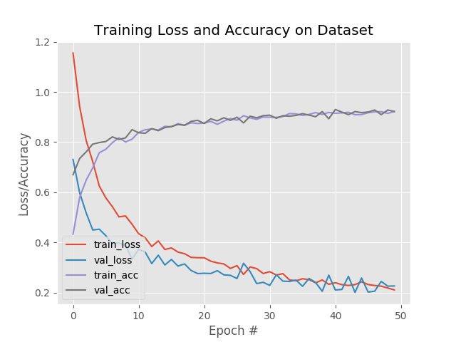
如您所见，在体育数据集上对 ResNet50 进行微调后，我们获得了约 94% 的准确率。 检查我们的模型目录，我们可以看到微调模型和标签二值化器已经序列化到磁盘：

使用 Keras 进行视频分类和滚动预测平均

=================================================================================

我们现在准备通过滚动预测精度使用 Keras 实现视频分类！ 为了创建这个脚本，我们将利用视频的时间特性，特别是假设视频中的后续帧将具有相似的语义内容。 通过执行滚动预测准确性，我们将能够“平滑”预测并避免“预测闪烁”。 让我们开始吧——打开 predict_video.py 文件并插入以下代码：

import the necessary packages

from tensorflow.keras.models import load_model

from collections import deque

import numpy as np

import argparse

import pickle

import cv2

construct the argument parser and parse the arguments

ap = argparse.ArgumentParser()

ap.add_argument(“-m”, “–model”, required=True,

help=“path to trained serialized model”)

ap.add_argument(“-l”, “–label-bin”, required=True,

help=“path to label binarizer”)

ap.add_argument(“-i”, “–input”, required=True,

help=“path to our input video”)

ap.add_argument(“-o”, “–output”, required=True,

help=“path to our output video”)

ap.add_argument(“-s”, “–size”, type=int, default=128,

help=“size of queue for averaging”)

args = vars(ap.parse_args())

加载必要的包和模块。 特别是，我们将使用 Python 集合模块中的 deque 来协助我们的滚动平均算法。

然后，解析五个命令行参数，其中四个是必需的：

–model ：从我们之前的训练步骤生成的输入模型的路径。

–label-bin ：前一个脚本生成的序列化 pickle 格式标签二值化器的路径。

–input ：用于视频分类的输入视频的路径。

–output ：我们将保存到磁盘的输出视频的路径。

–size ：滚动平均队列的最大大小（默认为 128）。 对于稍后的一些示例结果，我们将大小设置为 1，以便不执行平均。

有了我们的导入和命令行 args ，我们现在准备执行初始化：

load the trained model and label binarizer from disk

print(“[INFO] loading model and label binarizer…”)

model = load_model(args[“model”])

lb = pickle.loads(open(args[“label_bin”], “rb”).read())

initialize the image mean for mean subtraction along with the

predictions queue

mean = np.array([123.68, 116.779, 103.939][::1], dtype=“float32”)

Q = deque(maxlen=args[“size”])

加载我们的模型和标签二值化器。

然后设置我们的平均减法值。 我们将使用双端队列来实现我们的滚动预测平均。

我们的双端队列 Q 使用等于 args[“size”] 值的 maxlen 初始化。

让我们初始化我们的 cv2.VideoCapture 对象并开始循环视频帧：

initialize the video stream, pointer to output video file, and

frame dimensions

vs = cv2.VideoCapture(args[“input”])

writer = None

(W, H) = (None, None)

loop over frames from the video file stream

while True:

read the next frame from the file

(grabbed, frame) = vs.read()

if the frame was not grabbed, then we have reached the end

of the stream

if not grabbed:

break

if the frame dimensions are empty, grab them

if W is None or H is None:

(H, W) = frame.shape[:2]

抓取一个指向我们的输入视频文件流的指针。 我们使用 OpenCV 中的 VideoCapture 类从我们的视频流中读取帧。

然后，将我们的视频编写器和维度初始化为 None。

开始我们的视频分类 while 循环。

首先，我们抓取一个帧。 如果帧没有被抓取，那么我们已经到达了视频的结尾，此时我们将中断循环。

如果需要，然后设置我们的框架尺寸。 让我们预处理我们的框架：

clone the output frame, then convert it from BGR to RGB

ordering, resize the frame to a fixed 224x224, and then

perform mean subtraction

output = frame.copy()

frame = cv2.cvtColor(frame, cv2.COLOR_BGR2RGB)

frame = cv2.resize(frame, (224, 224)).astype(“float32”)

frame -= mean

我们的框架副本用于输出目的。

然后，我们使用与训练脚本相同的步骤对帧进行预处理，包括：

​ 交换颜色通道。

​ 调整为 224×224px。

​ 平均减法。

接下来是帧分类推理和滚动预测平均：

make predictions on the frame and then update the predictions

queue

preds = model.predict(np.expand_dims(frame, axis=0))[0]

Q.append(preds)

perform prediction averaging over the current history of

previous predictions

results = np.array(Q).mean(axis=0)

i = np.argmax(results)

label = lb.classes_[i]

对当前帧进行预测。 预测结果通过第 64 行添加到 Q。

从那里，对 Q 历史执行预测平均，从而为滚动平均值生成一个类标签。 分解后，这些线在平均预测中找到具有最大对应概率的标签。

现在我们有了结果标签，让我们注释我们的输出帧并将其写入磁盘：

自我介绍一下，小编13年上海交大毕业，曾经在小公司待过，也去过华为、OPPO等大厂，18年进入阿里一直到现在。

深知大多数Python工程师，想要提升技能，往往是自己摸索成长或者是报班学习，但对于培训机构动则几千的学费，着实压力不小。自己不成体系的自学效果低效又漫长，而且极易碰到天花板技术停滞不前！

因此收集整理了一份《2024年Python开发全套学习资料》，初衷也很简单，就是希望能够帮助到想自学提升又不知道该从何学起的朋友，同时减轻大家的负担。

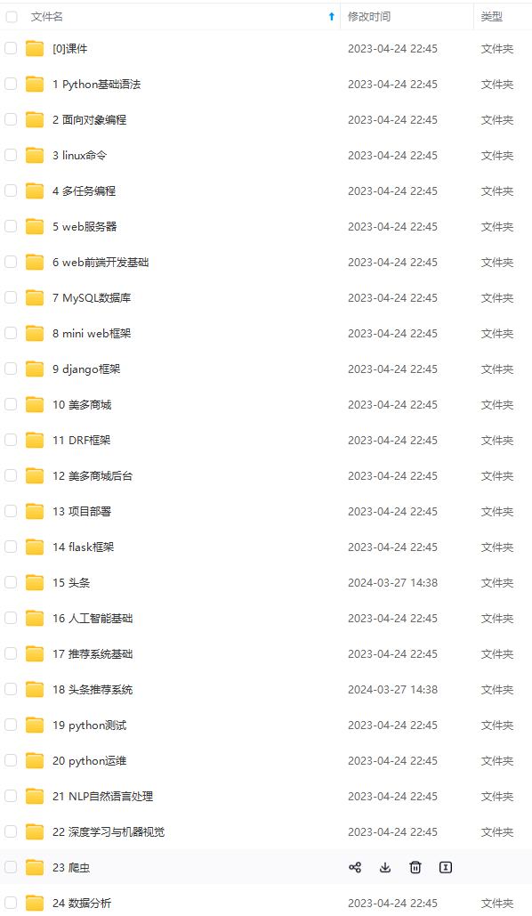
既有适合小白学习的零基础资料，也有适合3年以上经验的小伙伴深入学习提升的进阶课程，基本涵盖了95%以上Python开发知识点，真正体系化！

由于文件比较大，这里只是将部分目录大纲截图出来，每个节点里面都包含大厂面经、学习笔记、源码讲义、实战项目、讲解视频，并且后续会持续更新

如果你觉得这些内容对你有帮助，可以添加V获取：vip1024c （备注Python）

感谢每一个认真阅读我文章的人，看着粉丝一路的上涨和关注，礼尚往来总是要有的：

①　2000多本Python电子书（主流和经典的书籍应该都有了）

②　Python标准库资料（最全中文版）

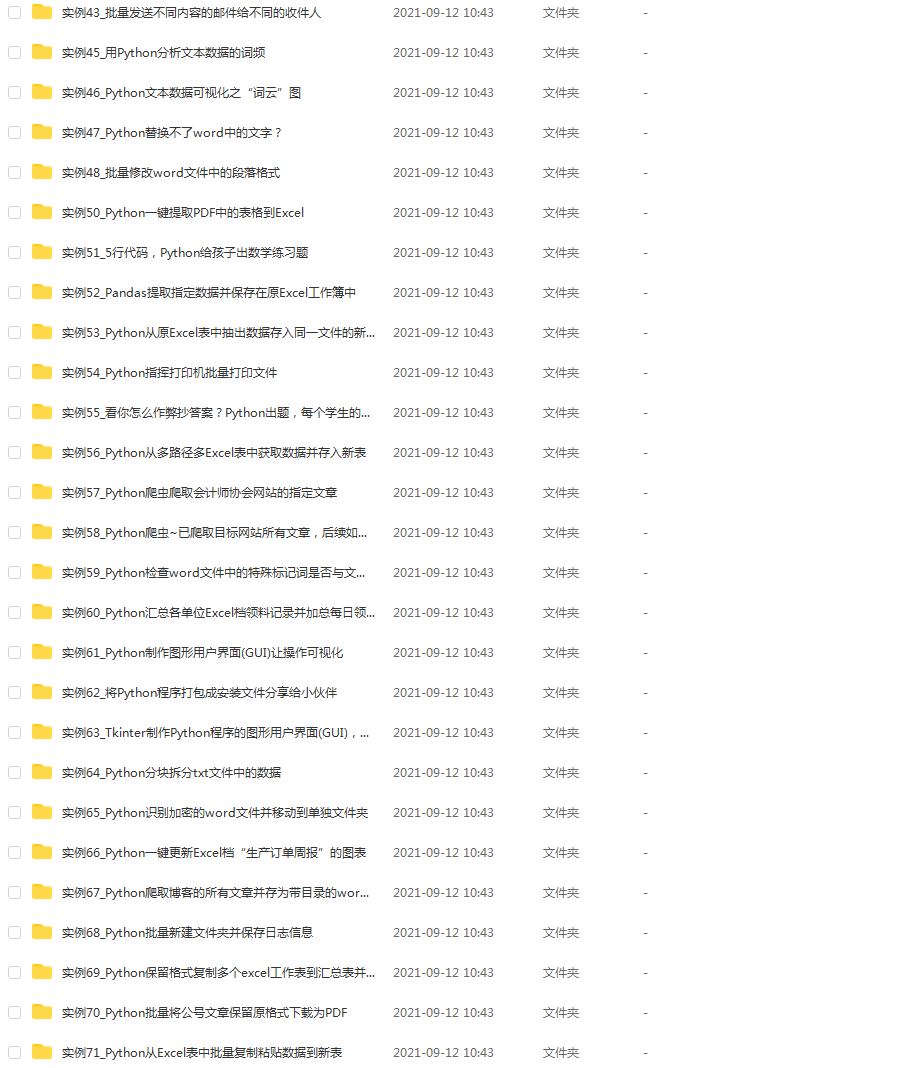
③　项目源码（四五十个有趣且经典的练手项目及源码）

④　Python基础入门、爬虫、web开发、大数据分析方面的视频（适合小白学习）

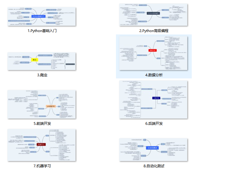
⑤ Python学习路线图（告别不入流的学习）

一个人可以走的很快，但一群人才能走的更远。不论你是正从事IT行业的老鸟或是对IT行业感兴趣的新人，都欢迎扫码加入我们的的圈子（技术交流、学习资源、职场吐槽、大厂内推、面试辅导），让我们一起学习成长！

6381401c05e862fe4e9.png)

既有适合小白学习的零基础资料，也有适合3年以上经验的小伙伴深入学习提升的进阶课程，基本涵盖了95%以上Python开发知识点，真正体系化！

由于文件比较大，这里只是将部分目录大纲截图出来，每个节点里面都包含大厂面经、学习笔记、源码讲义、实战项目、讲解视频，并且后续会持续更新

如果你觉得这些内容对你有帮助，可以添加V获取：vip1024c （备注Python）
[外链图片转存中…(img-YU83GgSO-1712958403704)]

感谢每一个认真阅读我文章的人，看着粉丝一路的上涨和关注，礼尚往来总是要有的：

①　2000多本Python电子书（主流和经典的书籍应该都有了）

②　Python标准库资料（最全中文版）

③　项目源码（四五十个有趣且经典的练手项目及源码）

④　Python基础入门、爬虫、web开发、大数据分析方面的视频（适合小白学习）

⑤ Python学习路线图（告别不入流的学习）

一个人可以走的很快，但一群人才能走的更远。不论你是正从事IT行业的老鸟或是对IT行业感兴趣的新人，都欢迎扫码加入我们的的圈子（技术交流、学习资源、职场吐槽、大厂内推、面试辅导），让我们一起学习成长！
[外链图片转存中…(img-VOm3OSx0-1712958403704)]