


直接学习目标:
- 了解数字图像的基本概念
- 了解医学图像的特点和成像方式
- 掌握读取图像和显示图像的方法
- 掌握获取图像特征的方法
直方图概念
- 直方图是图像灰度出现次数的统计分布,反映图像的灰度分布特征;
- 横轴代表灰度范围,纵轴代表每个灰度出现的次数
练习题1

# 读取图像
img = cv2.imread('data/MRI.png')

# 确保图像是灰度图,如果不是则转换为灰度图
if len(img.shape) > 2 and img.shape[2] == 3:
    img_gray = cv2.cvtColor(img, cv2.COLOR_BGR2GRAY)
else:
    img_gray = img

# 显示图像
plt.figure(figsize=(3,3))
plt.imshow(cv2.cvtColor(img, cv2.COLOR_BGR2RGB))  # OpenCV默认使用BGR,而matplotlib使用RGB
plt.title('Original Image')
plt.axis('off')  # 关闭坐标轴
plt.show()计算直方图并画出直方图(利用已有函数自己实现)
def GrayHist(img):
    # 计算灰度直方图
    height, width = img.shape[:2]
    grayHist = np.zeros([256], np.uint64)
    for i in range(height):
        for j in range(width):
            grayHist[img[i][j]] += 1

    # 归一化直方图
    grayHist_norm = grayHist.astype('float32') / grayHist.max()

    # 绘制直方图
    plt.figure(figsize=(6, 3))
    plt.plot(grayHist_norm, color='g')
    plt.xlim([0, 256])
    plt.title('Grayscale Histogram')
    plt.xlabel('Pixel Intensity')
    plt.ylabel('Normalized Frequency')
    plt.show()
    return grayHist_norm

# 计算并显示灰度直方图
grayHist_norm = GrayHist(img)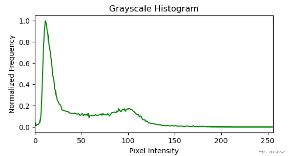
输出图像属性
# 输出图像的属性
height, width, channels = img.shape
print(f'分辨率: {width} x {height}')
print(f'通道数: {channels}')
print("图像行数:",img.shape[0])
print("图像列数:",img.shape[1])
print("图像通道数:",img.shape[2])
print("图像像素数:",img.size)
print("图像数据类型:",img.dtype)
print("图像形状信息:",img.shape)
直接调用函数计算直方图
# 直接调用函数计算直方图
hist = cv2.calcHist([img], [0], None, [256], [0,256])

# 绘制直方图
plt.figure(figsize=(6,4))
plt.title("Grayscale Histogram")
plt.xlabel("Bins")
plt.ylabel("# of Pixels")
plt.plot(hist, color='b')
plt.xlim([1, 256])
plt.ylim([0, 3500])  # 设置y轴范围
plt.grid(True)  # 添加网格线
plt.show()
打开DICOM图像
# 打开并显示图像
img3 = 'data/CT.dcm'
ds = pydicom.read_file(img3)
dcm = ds.pixel_array
plt.figure(figsize=(3,3))
plt.imshow(dcm,cmap = 'gray') # 显示灰度图像
plt.show()

# 显示图像信息
print("图像尺寸为:长",ds.Rows,"宽", ds.Columns)
# 显示患者信息
def PatientInformation(ds):#ds 是字典结构
    information={}
    information['PatientID'] = ds.PatientID
    information['PatientName'] = ds.PatientName
    information['PatientBirthDate'] = ds.PatientBirthDate
    information['PatientSex'] = ds.PatientSex
    information['StudyID'] = ds.StudyID
    information['StudyDate'] = ds.StudyDate
    information['InstitutionName'] = ds.InstitutionName
    return information
s = PatientInformation(ds)
print('患者ID:',s['PatientID'])
print('患者姓名:',s['PatientName'])
print('患者生日:',s['PatientBirthDate'])
print('患者性别:',s['PatientSex'])
print('研究标识符:',s['StudyID'])
print('研究日期:',s['StudyDate'])
print('机构名称:',s['InstitutionName'])
画出DICOM图像的直方图
ds.image = ds.pixel_array #将DICOM像素值转换为标准化的灰度范围

img2 = ds.pixel_array
cv2.imwrite('CT.jpg',img2)#保存为文件存储格式
img2 = cv2.imread('CT.jpg' ,cv2.IMREAD_GRAYSCALE)#读取灰度图
hist = cv2.calcHist([img2], [0], None, [256], [0, 256])
plt.plot(hist)
# 显示直方图
plt.xlabel('Pixel Va lue')
plt.ylabel('Frequency')
plt.title('CT Image Histogram')
plt.show()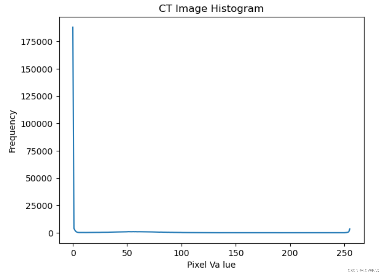
根据图像的最大最小灰度值绘制图像直方图
# 根据图像的最大最小灰度值绘制图像直方图
# CT图像通常具有较高的灰度级范围
# 利用ITK库读取dicom图像灰度值
import SimpleITK as itk
seg = itk.ReadImage('data/CT.dcm')
segimg = itk.GetArrayFromImage(seg)
print(segimg.min(),segimg.max())
hist = cv2.calcHist([img2],[0],None,[3774],[-2048,1727])
plt.plot(hist)

print(ds.RescaleSlope)
print(ds.RescaleIntercept)
# 打印图像HU值
HU=np.dot(segimg,ds.RescaleSlope)+ds.RescaleSlope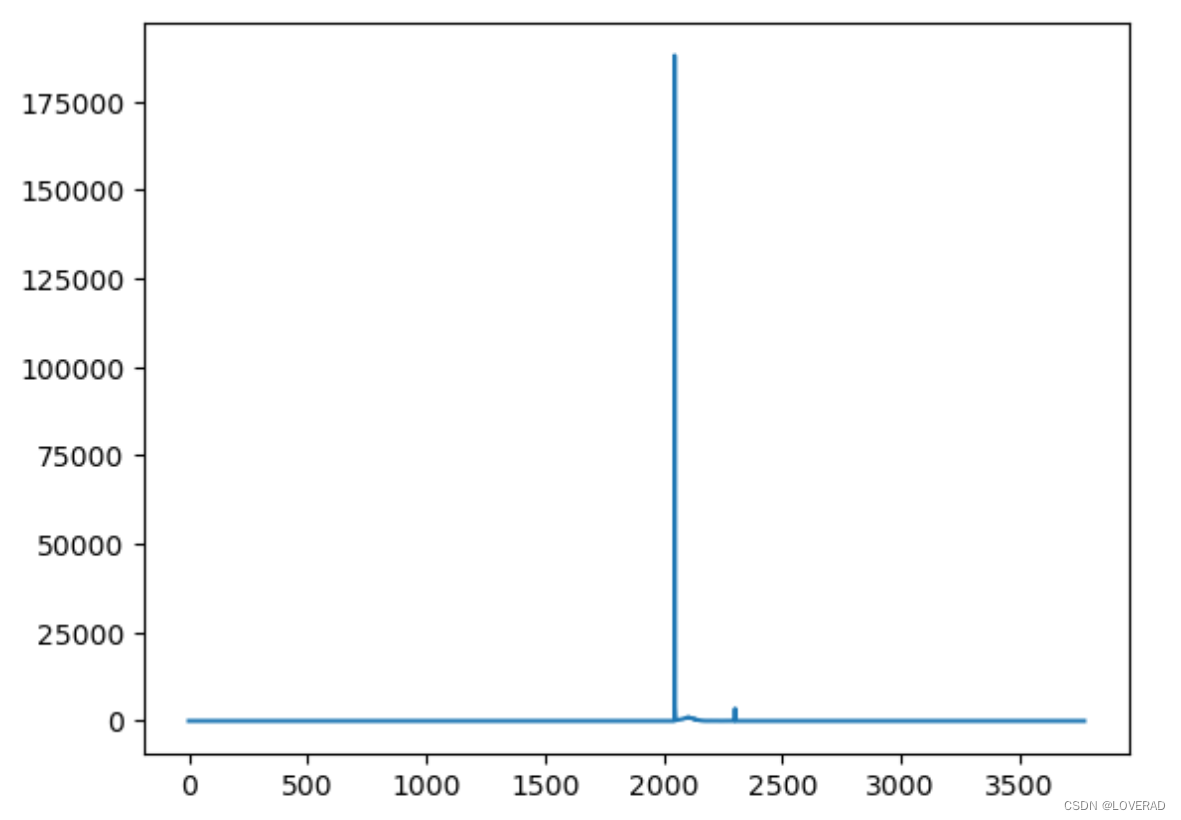
练习题2

调用OpenCV实现直方图均衡
import cv2
import matplotlib.pyplot as plt
import pydicom
import numpy as np

img = cv2.imread("data/brainMRI.jpg", cv2.IMREAD_GRAYSCALE ) #调用opencv库读取灰度图像
plt.figure(figsize=(8,8))
equ = cv2.equalizeHist(img) #调用opencv库实现直方图均衡,equ是增强后的图像

plt.subplot( 2, 2, 1 )
plt.hist(img.ravel(),256)#img.ravel()图像信息点进行统计,opencv画直方图
plt.title("Origin")

plt.subplot( 2, 2, 2 )
plt.hist(equ.ravel(),256)
plt.title("Equalization")

plt.subplot( 2, 2, 3 )
plt.imshow( img, cmap = 'gray' )#cmap 设置灰度颜色
plt.title( 'Origin' )

plt.subplot( 2, 2, 4 )
plt.imshow( equ, cmap = 'gray' )
plt.title( 'Equalization' )
plt.show()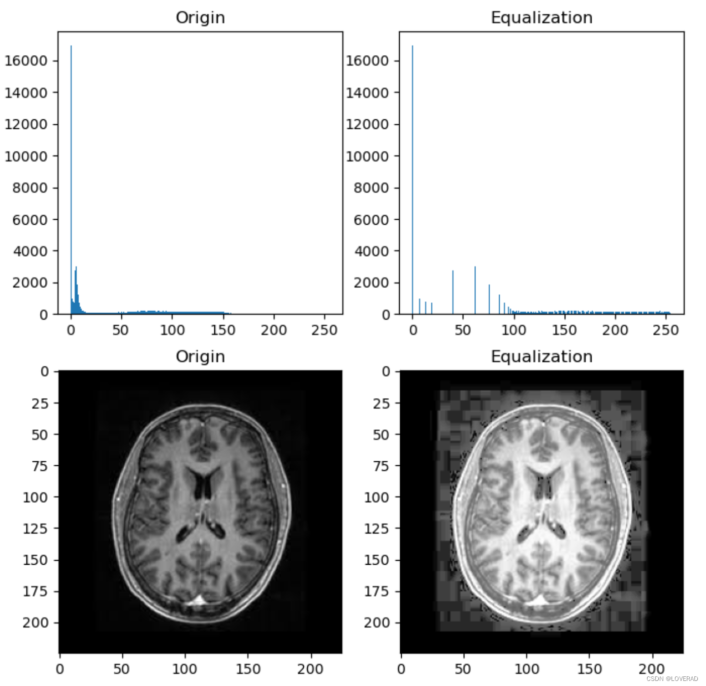
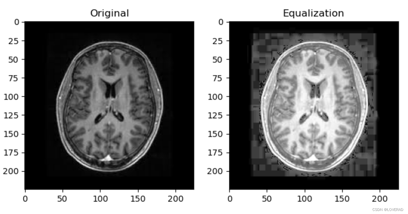
实现直方图均衡(利用已有函数,自己实现)
import cv2
import numpy as np
import matplotlib.pyplot as plt

def histogram_equalization(img):
    # 计算图像的直方图
    hist = cv2.calcHist([img], [0], None, [256], [0,256])

    # 计算累积分布函数 (CDF)
    cdf = hist.cumsum()
    cdf_normalized = cdf * hist.max() / cdf.max()

    # 创建一个映射函数,将原始像素值映射到新的像素值
    cdf_m = np.ma.masked_equal(cdf, 0)
    cdf_m = (cdf_m - cdf_m.min()) * 255 / (cdf_m.max() - cdf_m.min())
    cdf = np.ma.filled(cdf_m, 0).astype('uint8')

    # 使用映射函数来获取均衡化后的图像
    img_equalized = cdf[img]

    return img_equalized

# 读取图像
img = cv2.imread('data/brainMRI.jpg', cv2.IMREAD_GRAYSCALE)

# 进行直方图均衡化
img_equalized = histogram_equalization(img)

# 显示原始图像和均衡化后的图像
plt.figure(figsize=(8,8))

plt.subplot( 2, 2, 1 )
plt.imshow(img, cmap = plt.cm.gray)
plt.title('Original')

plt.subplot( 2, 2, 2 )
plt.imshow(img_equalized, cmap = plt.cm.gray)
plt.title('Equalization')

plt.show()
实现图像亮度增强,反转
import cv2
import numpy as np
import matplotlib.pyplot as plt

# 读取图像
img = cv2.imread('data/brainMRI.jpg', cv2.IMREAD_GRAYSCALE)

# 增强图像亮度
bright_img = cv2.convertScaleAbs(img, alpha=1, beta=50)

# 反转图像
invert_img = cv2.bitwise_not(img)

# 显示原始图像、增强亮度后的图像和反转后的图像
plt.figure(figsize=(12,12))

plt.subplot(1, 3, 1)
plt.imshow(img, cmap='gray')
plt.title('Original Image')

plt.subplot(1, 3, 2)
plt.imshow(bright_img, cmap='gray')
plt.title('Bright Image')

plt.subplot(1, 3, 3)
plt.imshow(invert_img, cmap='gray')
plt.title('Invert Image')

plt.show()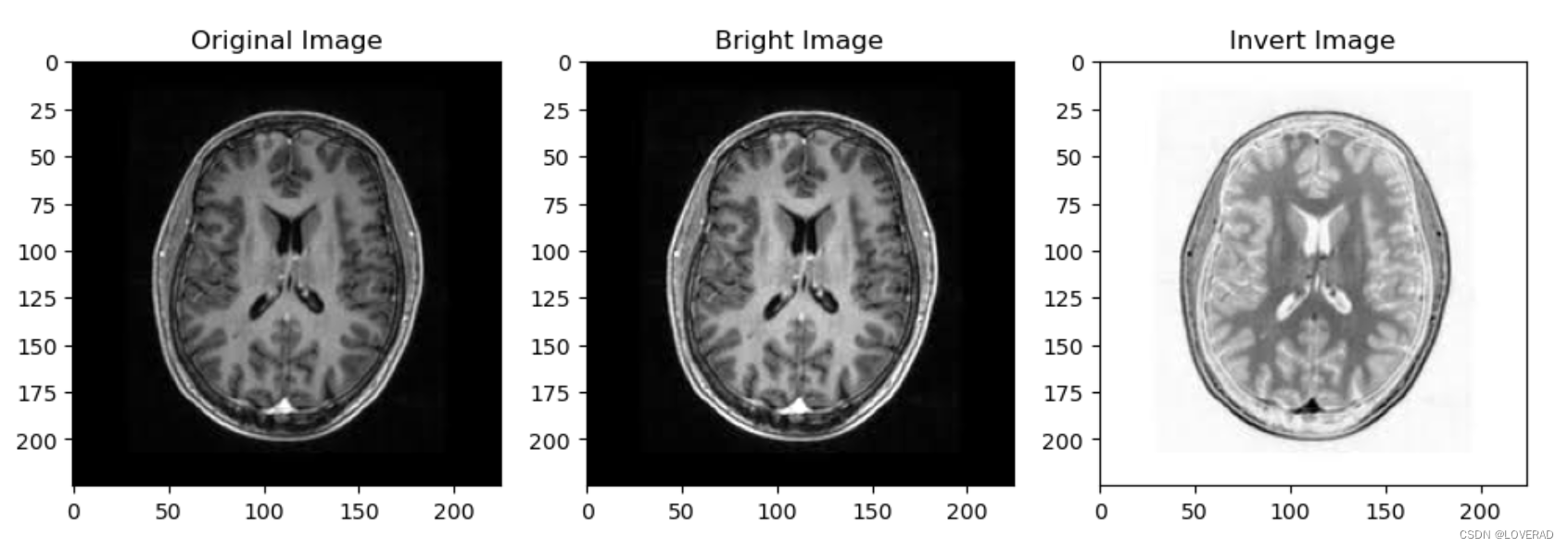
### 利用线性变换进行对比增强(可进行shepp loan phantom图像增强)
import cv2
import numpy as np
import matplotlib.pyplot as plt

# 读取图像
img = cv2.imread('data/MRI.jpg', cv2.IMREAD_GRAYSCALE)

# 获取图像的高度和宽度
height, width = img.shape

# 创建一个新的图像数组,用于存储处理后的图像
result = np.zeros_like(img, dtype=np.uint8)
# 遍历图像的每个像素
for i in range(height):
    for j in range(width):
        # 应用线性变换
        gray = int(img[i, j] * 1.5)

        # 如果结果大于255,则将其设置为255
        if gray > 255:
            gray = 255
        else:
            # 否则,保持结果值不变
            pass
        # 将处理后的像素值存储到result图像中
        result[i, j] = gray

# 显示原始图像和处理后的图像
plt.figure(figsize=(8, 4))

# 显示原始图像
plt.subplot(1, 2, 1)
plt.imshow(img, cmap='gray')
plt.title('Original Image')
plt.axis('off')

# 显示处理后的图像
plt.subplot(1, 2, 2)
plt.imshow(result, cmap='gray')
plt.title('Processed Image')
plt.axis('off')

plt.show()
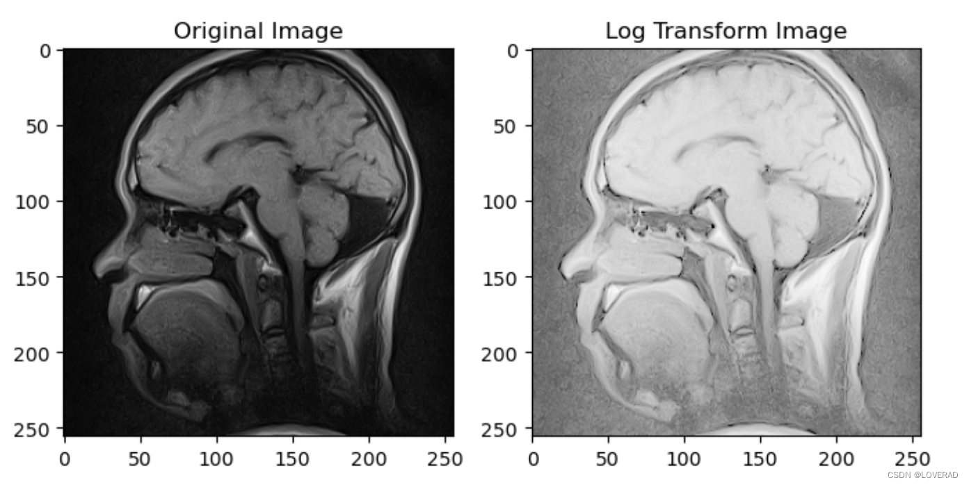
### 实现一种非线性灰度变换
import cv2
import numpy as np
import matplotlib.pyplot as plt
# 是灰度图像的对数变换。对数变换是一种非线性变换,通常用于扩展图像中较暗的像素值,同时压缩更亮的像素值,从而改善图像的对比度。

# 读取图像
img = cv2.imread('data/MRI.png', cv2.IMREAD_GRAYSCALE)

# 定义对数变换函数
def log_transform(c, img):
    output = c * np.log(1.0 + img)
    output = np.uint8(output + 0.5)
    return output

# 计算常数 c
c = 255 / np.log(1 + np.max(img))

# 进行灰度对数变换
img_log = log_transform(c, img)

# 显示原始图像和变换后的图像
plt.figure(figsize=(8,8))

plt.subplot(1, 2, 1)
plt.imshow(img, cmap='gray')
plt.title('Original Image')

plt.subplot(1, 2, 2)
plt.imshow(img_log, cmap='gray')
plt.title('Log Transform Image')

plt.show()


 被折叠的 条评论
为什么被折叠?
被折叠的 条评论
为什么被折叠?
 到【灌水乐园】发言


