


这个版本最显著的特点是,在保留打车功能的同时,完全没有任何广告的干扰,而且,这个版本的应用体积非常小巧。并且地图也是在实时更新的。
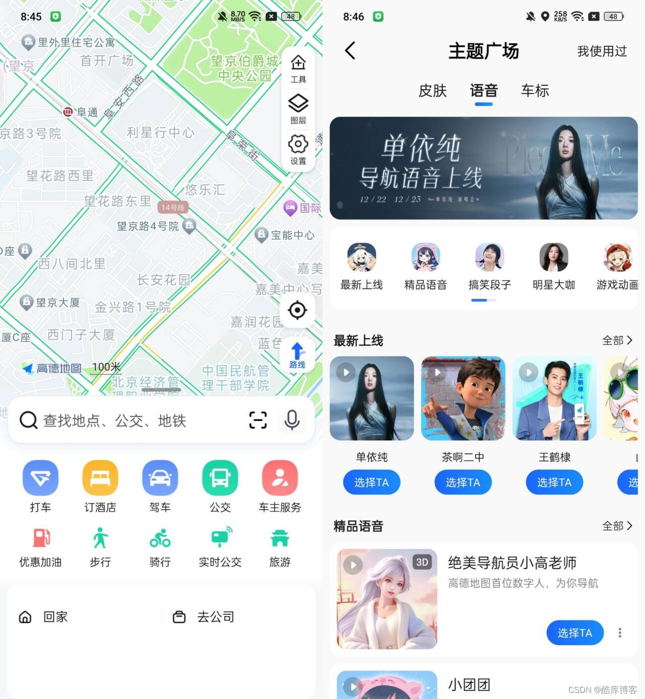
和标准版的高德地图相比几乎没有什么区别,在支持驾车、骑行、公交地铁、步行等导航模式方面表现出色,可以享受到(如郭德纲、小团团、林志玲等等语音包,并且全部是免费的!)。
并且各位老司机最需要的电子狗的功能也是有的,可以一键检测附近所有的电子摄像头,带红绿灯倒计时!
这个版本最显著的特点是,在保留打车功能的同时,完全没有任何广告的干扰,而且,这个版本的应用体积非常小巧。并且地图也是在实时更新的。
和标准版的高德地图相比几乎没有什么区别,在支持驾车、骑行、公交地铁、步行等导航模式方面表现出色,可以享受到(如郭德纲、小团团、林志玲等等语音包,并且全部是免费的!)。
并且各位老司机最需要的电子狗的功能也是有的,可以一键检测附近所有的电子摄像头,带红绿灯倒计时!
 4552
534
169
4552
534
169


 被折叠的 条评论
为什么被折叠?
被折叠的 条评论
为什么被折叠?
 到【灌水乐园】发言


