Python 最大功率点跟踪（MPPT）模拟计算——blog15

写在前面

MPPT，即最大功率点跟踪，是一种用于太阳能光伏系统中的电子控制技术。太阳能光伏系统中，太阳能电池板会根据光照强弱的变化产生不同的电压和电流输出。而最大功率点跟踪技术就是通过调整电池板的工作点，使其输出的功率达到最大值。

最大功率点跟踪技术主要通过电子控制器来实现，电子控制器会监测太阳能电池板的输出电压和电流，并根据预设的算法和逻辑来调整电池板的工作点。当光照强度较弱时，控制器会提高电池板的输出电压，使其工作在输出功率最大的点上；当光照强度较强时，控制器会降低电池板的输出电压，以防止过载。

MPPT技术的应用能够显著提高太阳能光伏系统的转换效率，使其能够更充分地利用光能。与传统的固定工作点技术相比，MPPT技术能够在不同光照条件下实时跟踪光伏系统的最大功率点，从而提高系统的发电效率。

项目开始

准备工作

import numpy as np
import matplotlib.pyplot as plt

纹波电流计算

Vin_list = [10, 15, 20, 10, 15, 20, 10, 15, 20]
Vout_list = [20, 30, 40, 11.67, 14.29, 16.67, 23.33, 30, 40]
Iout = 2  # 负载电流（安培）
fs = 100000  # 开关频率（赫兹）
L = 50e-6  # 电感值（亨利）
# 计算占空比

for t in range(len(Vin_list)):

    D = Vout_list[t] / Vin_list[t]
# 计算纹波电流
    delta_I = (Vin_list[t] - Vout_list[t]) * D / (fs * L)
# 计算最大最小电流
    I_max = Iout + delta_I / 2
    I_min = Iout - delta_I / 2
# 创建时间数组（一个周期内）
    x = np.linspace(0, 1 / fs, num=1000)
# 计算电流波形
    i_L = I_min + (I_max - I_min) * (1 - np.exp(-x / (D / fs * L))) / (1 - np.exp(-1 / (fs * L)))
# 绘制图像
    plt.subplot(len(Vin_list), 1, t+1)
    plt.plot(x * 1e6, i_L)
    plt.xlabel('T(us)')
    plt.ylabel('IC (A)')
    plt.title('IBC')
    plt.grid(True)

plt.show()

fft

# 定义仿真参数
T = 1e-4
t = np.arange(0, 5*T, T)
Vin = 40
Iin = np.sin(2*np.pi*50*t)
Vout = np.zeros(len(t))
Duty = np.zeros(len(t))
Pout = np.zeros(len(t))
Vref = 20
# 计算辅助变量
L = 220 * 1e-6
C = 220 * 1e-6
R = 10
alpha = (Vin - Vref) / Vin
beta = (Vref * R) / (Vin * L)
# 开始模拟
for i in range(1, len(t)):
    # 计算功率和控制量
    Pout[i] = Vout[i-1] * Iin[i-1]
    Duty[i] = alpha + beta * Iin[i-1]
    # 限幅
    Duty[i] = max(min(Duty[i], 1), 0)
    # 更新电压和电流
    if Pout[i] > Pout[i-1]:
        Vout[i] = Vout[i-1] + (Duty[i] * Vin - Vout[i-1]) * T / (L * C)
    else:
        Vout[i] = Vout[i-1] - (Vout[i-1] / (L * R)) * T
# 绘制图像
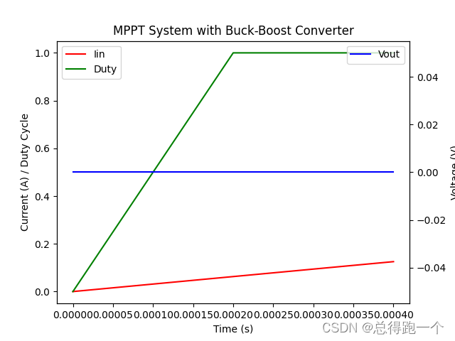
fig, ax1 = plt.subplots()
ax2 = ax1.twinx()
ax1.plot(t, Iin, 'r', label='Iin')
ax1.plot(t, Duty, 'g', label='Duty')
ax2.plot(t, Vout, 'b', label='Vout')
ax1.set_xlabel('Time (s)')
ax1.set_ylabel('Current (A) / Duty Cycle')
ax2.set_ylabel('Voltage (V)')
ax1.set_title('MPPT System with Buck-Boost Converter')
ax1.legend(loc='upper left')
ax2.legend(loc='upper right')
plt.show()

交错升降压

# 定义仿真参数
T = 1e-4
t = np.arange(0, 5*T, T)
Vin = 40
Iin = np.sin(2*np.pi*50*t)
Vout = np.zeros(len(t))
Duty = np.zeros(len(t))
Pout = np.zeros(len(t))
Vref = 20

# 计算辅助变量
L = 220 * 1e-6
C = 220 * 1e-6
R = 10
alpha = (Vin - Vref) / Vin
beta = (Vref * R) / (Vin * L)
# 开始模拟
for i in range(1, len(t)):
    # 计算功率和控制量
    Pout[i] = Vout[i-1] * Iin[i-1]
    Duty[i] = alpha + beta * Iin[i-1]
    # 限幅
    Duty[i] = max(min(Duty[i], 1), 0)
    # 更新电压和电流
    if Pout[i] > Pout[i-1]:
        Vout[i] = Vout[i-1] + (Duty[i] * Vin - Vout[i-1]) * T / (L * C)
    else:
        Vout[i] = Vout[i-1] - (Vout[i-1] / (L * R)) * T
# 绘制图像
fig, ax1 = plt.subplots()
ax2 = ax1.twinx()
ax1.plot(t, Iin, 'r', label='Iin')
ax1.plot(t, Duty, 'g', label='Duty')
ax2.plot(t, Vout, 'b', label='Vout')
ax1.set_xlabel('Time (s)')
ax1.set_ylabel('Current (A) / Duty Cycle')
ax2.set_ylabel('Voltage (V)')
ax1.set_title('MPPT System with Buck-Boost Converter')
ax1.legend(loc='upper left')
ax2.legend(loc='upper right')
plt.show()

光伏侧电压变化

# 定义控制参数
Kp1 = 0.2
Ki1 = 0.05
Kp2 = 0.1
Ki2 = 0.02

# 定义仿真参数
T = 1e-4
t = np.arange(0, 5*T, T)
Vref = 200
Vpv = np.zeros(len(t))
Vbuck = np.zeros(len(t))
Ibuck = np.zeros(len(t))
Vboost = np.zeros(len(t))
Iboost = np.zeros(len(t))
# 开始模拟
for i in range(1, len(t)):
    # 计算误差和积分项
    e1 = Vref - Vpv[i-1]
    e2 = Vpv[i-1] - Vbuck[i-1]
    Iint1 = np.sum(e1 * T)
    Iint2 = np.sum(e2 * T)
    # 计算控制量
    Duty_buck = Kp1 * e1 + Ki1 * Iint1
    Duty_boost = Kp2 * e2 + Ki2 * Iint2
    # 限幅
    Duty_buck = max(min(Duty_buck, 1), 0)
    Duty_boost = max(min(Duty_boost, 1), 0)
    # 更新电压和电流
    Ibuck[i] = Duty_buck * 10
    Iboost[i] = Duty_boost * 10
    Vbuck[i] = Vbuck[i-1] + T * (10 - Ibuck[i-1]) / (220 * 1e-6)
    Vboost[i] = Vboost[i-1] + T * (Ibuck[i-1] - Iboost[i-1]) / (220 * 1e-6)
    Vpv[i] = Vpv[i-1] + T * (-(Vpv[i-1] * Ibuck[i-1]) / 1000)
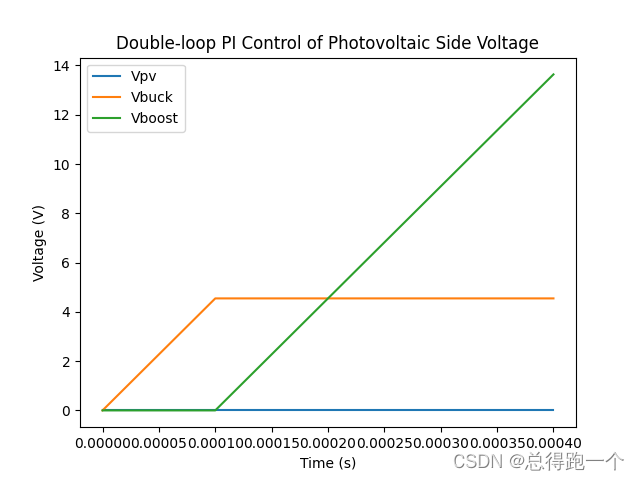
# 绘制图像
plt.plot(t, Vpv, label='Vpv')
plt.plot(t, Vbuck, label='Vbuck')
plt.plot(t, Vboost, label='Vboost')
plt.xlabel('Time (s)')
plt.ylabel('Voltage (V)')
plt.title('Double-loop PI Control of Photovoltaic Side Voltage')
plt.legend()
plt.show()

觉得有帮助的小伙伴还请点个关注

后续会持续分享 免费、高质量 的高校相关以及Python学习文章