关于银行信贷客户数据集的探索

本数据集来自一家德国银行，由加州大学霍夫曼教授于 2016 年收集整理，每条记录代表了一个接受银行信贷的客户，这也就说明了，这些客户都是通过了贷款申请的，通过可视化分析对数据进行初步探索，并利用聚类分析将客户分为不同的风险群体，由于数据集中缺乏直接的客户贷款风险标签，我们无法直接评估风险分类的准确性，因此，再次采用聚类分析（不考虑客户贷款风险特征），将数据分为四个类别，分类结果与实际相符，可以构建随机森林模型来识别风险分类的关键因素，虽然无法准确评估模型的精度，但该模型仍可作为初步风险评估的有效工具，从而提高风险识别的效率。

2.数据说明

字段	说明
Age	年龄
Sex	性别，male（男性），female（女性）
Job	职业，0 - 无技能且非常驻，1 - 无技能且常驻，2 - 有技能，3 - 高技能
Housing	住房类型：own（自有房产），rent（租房），free（免租赁）
Saving accounts	客户的储蓄账户状况 - little（少量），moderate（适中），quite rich（相对富裕），rich（富裕）
Checking account	支票账户，little（少量），moderate（适中），rich（富裕）
Credit amount	贷款金额，（单位：德国马克）
Duration	贷款期限，（单位：月）
Purpose	贷款用途，car（汽车），furniture/equipment（家具/设备），radio/TV（收音机/电视），domestic appliances（家用电器），repairs（修理），education（教育），business（商业），vacation/others（假期/其他）

3.Python库导入及数据读取

In [1]:

# 导入需要的库
import pandas as pd
import numpy as np
import seaborn as sns
import matplotlib.pyplot as plt
from sklearn.preprocessing import StandardScaler
from sklearn.cluster import KMeans
from sklearn.metrics import silhouette_score
from sklearn.model_selection import train_test_split
from sklearn.utils import resample
from sklearn.ensemble import RandomForestClassifier
from sklearn.metrics import classification_report,confusion_matrix

In [2]:

data = pd.read_csv("/home/mw/input/customer9878/german_credit_data.csv")

4.数据预览及数据处理

4.1数据预览

In [3]:

# 查看数据维度
data.shape

Out[3]:

(1000, 10)

In [4]:

# 查看数据信息
data.info()

<class 'pandas.core.frame.DataFrame'>
RangeIndex: 1000 entries, 0 to 999
Data columns (total 10 columns):
Id                  1000 non-null int64
Age                 1000 non-null int64
Sex                 1000 non-null object
Job                 1000 non-null int64
Housing             1000 non-null object
Saving accounts     817 non-null object
Checking account    606 non-null object
Credit amount       1000 non-null int64
Duration            1000 non-null int64
Purpose             1000 non-null object
dtypes: int64(5), object(5)
memory usage: 78.2+ KB

In [5]:

# 查看各列缺失值
data.isna().sum()

Out[5]:

Id                    0
Age                   0
Sex                   0
Job                   0
Housing               0
Saving accounts     183
Checking account    394
Credit amount         0
Duration              0
Purpose               0
dtype: int64

In [6]:

# 查看重复值
data.duplicated().sum()

Out[6]:

0

4.2数据处理

In [7]:

# 处理Saving accounts和Checking account中缺失值。
# 考虑到缺失值占比比较大，不建议直接删除，同样的，也不建议用众数填充，这样可能会改变数据情况，这里先用unknown填充。
data['Saving accounts'].fillna('unknown', inplace=True)
data['Checking account'].fillna('unknown', inplace=True)
data.isna().sum()

Out[7]:

Id                  0
Age                 0
Sex                 0
Job                 0
Housing             0
Saving accounts     0
Checking account    0
Credit amount       0
Duration            0
Purpose             0
dtype: int64

In [8]:

# 查看分类特征的唯一值
characteristic = ['Sex','Job','Housing','Saving accounts','Checking account','Purpose']
for i in characteristic:
    print(f'{i}:')
    print(data[i].unique())
    print('-'*50)

Sex:
['male' 'female']
--------------------------------------------------
Job:
[2 1 3 0]
--------------------------------------------------
Housing:
['own' 'free' 'rent']
--------------------------------------------------
Saving accounts:
['unknown' 'little' 'quite rich' 'rich' 'moderate']
--------------------------------------------------
Checking account:
['little' 'moderate' 'unknown' 'rich']
--------------------------------------------------
Purpose:
['radio/TV' 'education' 'furniture/equipment' 'car' 'business'
 'domestic appliances' 'repairs' 'vacation/others']
--------------------------------------------------

In [9]:

# 将 Id 修改为字符串类型
data['Id'] = data['Id'].astype(str)

5.数据探索

5.1客户基本情况分析

In [10]:

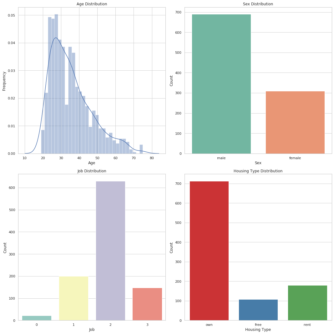
# 设置绘图风格
sns.set(style="whitegrid")
fig, axs = plt.subplots(2, 2, figsize=(15,15))
# 年龄分布
sns.distplot(data['Age'], kde=True, bins=30, ax=axs[0, 0])
axs[0, 0].set_title('Age Distribution')
axs[0, 0].set_xlabel('Age')
axs[0, 0].set_ylabel('Frequency')

# 性别分布
sns.countplot(x='Sex', data=data, palette='Set2', ax=axs[0, 1])
axs[0, 1].set_title('Sex Distribution')
axs[0, 1].set_xlabel('Sex')
axs[0, 1].set_ylabel('Count')

# 职业技能分布
sns.countplot(x='Job', data=data, palette='Set3', ax=axs[1, 0])
axs[1, 0].set_title('Job Distribution')
axs[1, 0].set_xlabel('Job')
axs[1, 0].set_ylabel('Count')

# 住房类型分布
sns.countplot(x='Housing', data=data, palette='Set1', ax=axs[1, 1])
axs[1, 1].set_title('Housing Type Distribution')
axs[1, 1].set_xlabel('Housing Type')
axs[1, 1].set_ylabel('Count')

plt.tight_layout()
plt.show()

通过上图可以得到如下结论：
1.客户年龄主要集中在较年轻的年龄段，可能表明年轻人更倾向于申请贷款。
2.男性客户数量高于女性客户数量。
3.工作位于2级的客户数量最多，0级的客户数量最少，可能是因为0级无技能且非常驻，银行不予贷款。
4.自有房产客户数量>租房客户数量>免租赁客户数量，这里免租赁客户指的是那些居住在无需支付租金的住所的人，比如住在政府提供的免费住宿或者亲戚朋友家里。

5.2客户经济情况分析

In [11]:

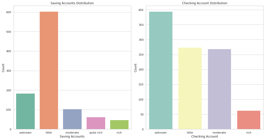
order_savings = ['unknown', 'little', 'moderate', 'quite rich', 'rich']
order_checking = ['unknown', 'little', 'moderate', 'rich']

fig, axs = plt.subplots(1, 2, figsize=(15,8))

# 储蓄账户状况分布
sns.countplot(x='Saving accounts', data=data, order=order_savings, palette='Set2', ax=axs[0])
axs[0].set_title('Saving Accounts Distribution')
axs[0].set_xlabel('Saving Accounts')
axs[0].set_ylabel('Count')

# 支票账户分布
sns.countplot(x='Checking account', data=data, order=order_checking, palette='Set3', ax=axs[1])
axs[1].set_title('Checking Account Distribution')
axs[1].set_xlabel('Checking Account')
axs[1].set_ylabel('Count')
plt.tight_layout()
plt.show()

通过上图，可以得知：
1.越有钱的客户越不容易选择贷款。
2.储蓄账户状况为少量的客户，贷款人数最多。
3.支票账户状况为未知、少量、中等贷款人数比较多，尤其是位置的客户是最多的，表明放款的时候，支票账户可能不是一个主要的考虑因素，才会导致未知数据占多数。

5.3客户贷款情况分析

In [12]:

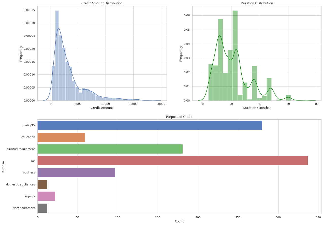
fig = plt.figure(figsize=(20,15))

# 创建2x2的图布局
ax1 = fig.add_subplot(2, 2, 1)
ax2 = fig.add_subplot(2, 2, 2)
ax3 = fig.add_subplot(2, 1, 2)

# 贷款金额分布
sns.distplot(data['Credit amount'], kde=True, bins=30, ax=ax1)
ax1.set_title('Credit Amount Distribution')
ax1.set_xlabel('Credit Amount')
ax1.set_ylabel('Frequency')

# 贷款期限分布
sns.distplot(data['Duration'], kde=True, bins=20, color='green', ax=ax2)
ax2.set_title('Duration Distribution')
ax2.set_xlabel('Duration (Months)')
ax2.set_ylabel('Frequency')

# 贷款用途分布
sns.countplot(y='Purpose', data=data, palette='muted', ax=ax3)
ax3.set_title('Purpose of Credit')
ax3.set_xlabel('Count')
ax3.set_ylabel('Purpose')

Out[12]:

Text(0, 0.5, 'Purpose')

通过上图，可以得知：
1.客户贷款主要倾向于申请中低额度的贷款，贷款期限也主要选择中短期。
2.客户贷款用途主要用于购买车、收音机/电视、家具/设备。

6.客户贷款风险评估

6.1数据预处理

In [13]:

# 因为需要进行聚类，所以需要对数据进行初步处理，这里对数值型数据，进行标准化，对分类变量处理为有序变量。
# 选择特征
features = ['Age', 'Sex', 'Job', 'Housing', 'Saving accounts', 'Checking account', 'Credit amount', 'Duration']
new_data = data[features].copy()

# 对类别型特征进行有序编码
new_data['Sex'] = new_data['Sex'].map({
    'female': 0,
    'male': 1})

new_data['Housing'] = new_data['Housing'].map({
    'free': 0,
    'rent': 1,
    'own': 2})

new_data['Saving accounts'] = new_data['Saving accounts'].map({
    'unknown': 0,
    'little': 1,
    'moderate': 2,
    'quite rich': 3,
    'rich': 4})

new_data['Checking account'] = new_data['Checking account'].map({
    'unknown': 0,
    'little': 1,
    'moderate': 2,
    'rich': 3})

# 标准化数值型特征
scaler = StandardScaler()
num_features = ['Age', 'Credit amount', 'Duration']
new_data[num_features] = scaler.fit_transform(new_data[num_features])

new_data.head(10)

Out[13]:

	Age	Sex	Job	Housing	Saving accounts	Checking account	Credit amount	Duration
0	2.766456	1	2	2	0	1	-0.745131	-1.236478
1	-1.191404	0	2	2	1	2	0.949817	2.248194
2	1.183312	1	1	2	1	0	-0.416562	-0.738668
3	0.831502	1	2	0	1	1	1.634247	1.750384
4	1.535122	1	2	0	1	1	0.566664	0.256953
5	-0.048022	1	1	0	0	0	2.050009	1.252574
6	1.535122	1	2	2	3	0	-0.154629	0.256953
7	-0.048022	1	3	1	1	2	1.303197	1.252574
8	2.238742	1	1	2	4	0	-0.075233	-0.738668
9	-0.663689	1	3	2	1	2	0.695681	0.754763

6.2划分高风险客户和低风险客户

In [14]:

# 模型选择：使用KMeans进行聚类
kmeans = KMeans(n_clusters=2, random_state=15)
clusters = kmeans.fit_predict(new_data)
# 将聚类结果添加到数据中
data['Risk Group'] = clusters
data.head(10)

Out[14]:

	Id	Age	Sex	Job	Housing	Saving accounts	Checking account	Credit amount	Duration	Purpose	Risk Group
0	0	67	male	2	own	unknown	little	1169	6	radio/TV	1
1	1	22	female	2	own	little	moderate	5951	48	radio/TV	0
2	2	49	male	1	own	little	unknown	2096	12	education	1
3	3	45	male	2	free	little	little	7882	42	furniture/equipment	0
4	4	53	male	2	free	little	little	4870	24	car	0
5	5	35	male	1	free	unknown	unknown	9055	36	education	0
6	6	53	male	2	own	quite rich	unknown	2835	24	furniture/equipment	1
7	7	35	male	3	rent	little	moderate	6948	36	car	0
8	8	61	male	1	own	rich	unknown	3059	12	radio/TV	1
9	9	28	male	3	own	little	moderate	5234	30	car	0

6.3两类客户之间对比

6.3.1基本情况对比

In [15]:

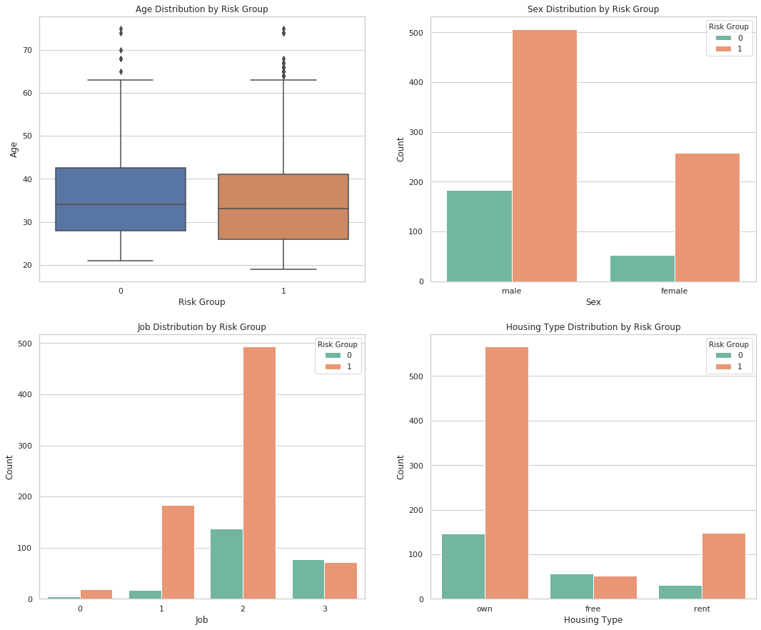
fig, axs = plt.subplots(2, 2, figsize=(18,15))

sns.boxplot(x='Risk Group', y='Age', data=data, ax=axs[0, 0])
axs[0, 0].set_title('Age Distribution by Risk Group')
axs[0, 0].set_xlabel('Risk Group')
axs[0, 0].set_ylabel('Age')

sns.countplot(x='Sex', hue='Risk Group', data=data, palette='Set2', ax=axs[0, 1])
axs[0, 1].set_title('Sex Distribution by Risk Group')
axs[0, 1].set_xlabel('Sex')
axs[0, 1].set_ylabel('Count')

sns.countplot(x='Job', hue='Risk Group', data=data, palette='Set2', ax=axs[1, 0])
axs[1, 0].set_title('Job Distribution by Risk Group')
axs[1, 0].set_xlabel('Job')
axs[1, 0].set_ylabel('Count')

sns.countplot(x='Housing', hue='Risk Group', data=data, palette='Set2', ax=axs[1, 1])
axs[1, 1].set_title('Housing Type Distribution by Risk Group')
axs[1, 1].set_xlabel('Housing Type')
axs[1, 1].set_ylabel('Count')

Out[15]:

Text(0, 0.5, 'Count')

6.3.2经济情况对比

In [16]:

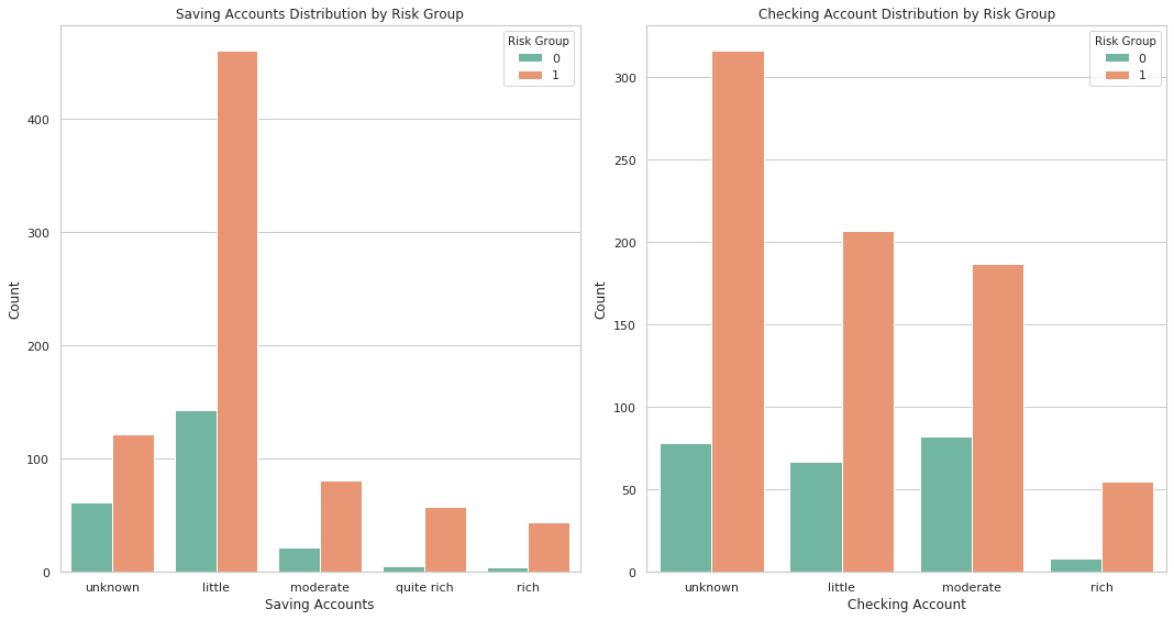
order_savings = ['unknown', 'little', 'moderate', 'quite rich', 'rich']
order_checking = ['unknown', 'little', 'moderate', 'rich']

fig, axs = plt.subplots(1, 2, figsize=(15,8))

sns.countplot(x='Saving accounts', hue='Risk Group', data=data, order=order_savings, palette='Set2', ax=axs[0])
axs[0].set_title('Saving Accounts Distribution by Risk Group')
axs[0].set_xlabel('Saving Accounts')
axs[0].set_ylabel('Count')

sns.countplot(x='Checking account', hue='Risk Group', data=data, order=order_checking, palette='Set2', ax=axs[1])
axs[1].set_title('Checking Account Distribution by Risk Group')
axs[1].set_xlabel('Checking Account')
axs[1].set_ylabel('Count')

plt.tight_layout()
plt.show()

6.3.3贷款情况对比

In [17]:

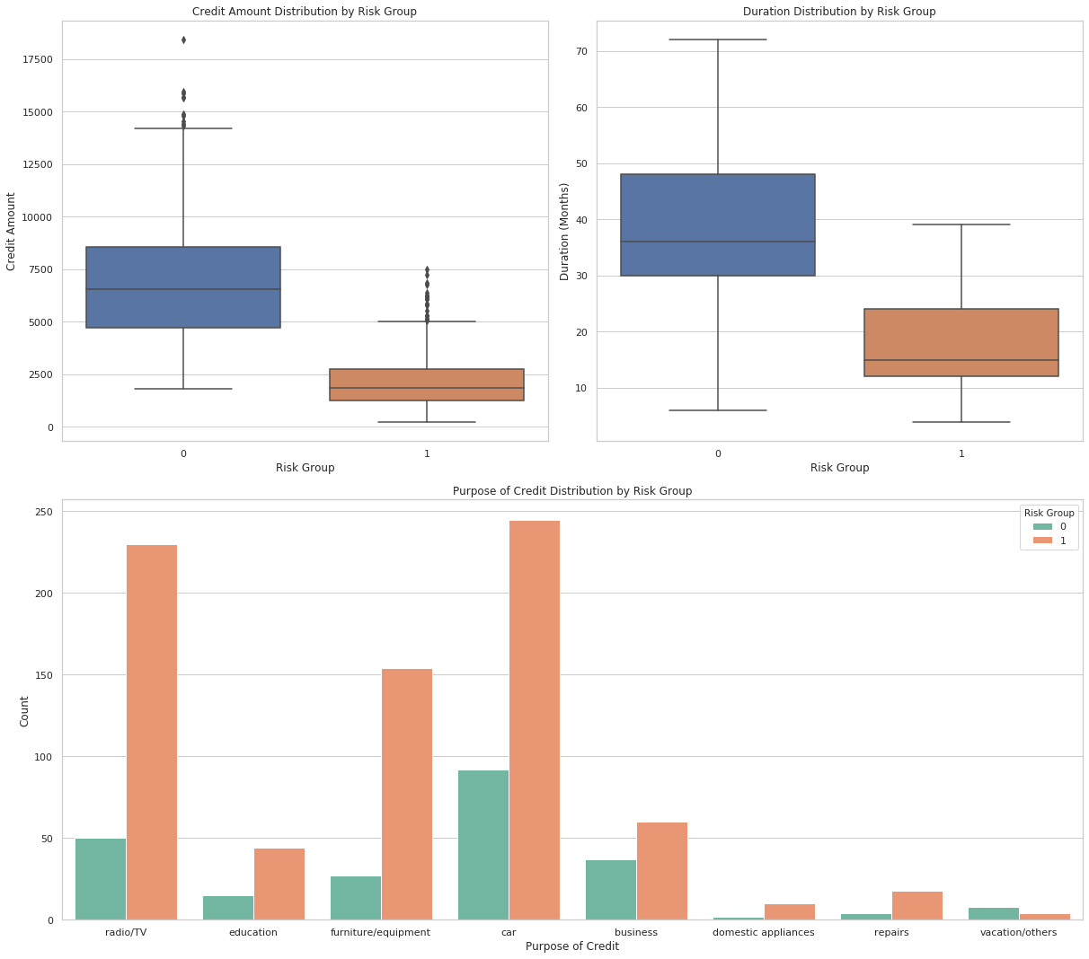
fig = plt.figure(figsize=(17,15))

# 创建2x2的图布局
ax1 = fig.add_subplot(2, 2, 1)
ax2 = fig.add_subplot(2, 2, 2)
ax3 = fig.add_subplot(2, 1, 2)

sns.boxplot(x='Risk Group', y='Credit amount', data=data, ax=ax1)
ax1.set_title('Credit Amount Distribution by Risk Group')
ax1.set_xlabel('Risk Group')
ax1.set_ylabel('Credit Amount')

sns.boxplot(x='Risk Group', y='Duration', data=data, ax=ax2)
ax2.set_title('Duration Distribution by Risk Group')
ax2.set_xlabel('Risk Group')
ax2.set_ylabel('Duration (Months)')

sns.countplot(x='Purpose', hue='Risk Group', data=data, palette='Set2', ax=ax3)
ax3.set_title('Purpose of Credit Distribution by Risk Group')
ax3.set_xlabel('Purpose of Credit')
ax3.set_ylabel('Count')

plt.tight_layout()
plt.show()

通过三类不同情况的分析，可以初步判断，0为高风险人群，1为低风险人群，原因如下：
1.类型1不仅借款金额远小于类型0，并且借款周期也远小于类型0，表明类型0的客户还款负担更重。
2.类型0虽然资金更加充足(储蓄账户状况、支票账户状况)，但是通过贷款用途可以看到，主要用于商业和购买车子(占比更大)，可以初步判断类型1中，有一些商人，从职业等级也能看出来，大部分在2和3，这一类人群，虽然有钱，但是开销也大，因此风险比类型1高。
因此，可以认为类型1属于低风险用户，类型0属于高风险用户，因为没有违约数据，这里只能通过聚类来简单划分一下。

7.用户画像分析

这步与上一步不同，我这里并没有将风险评估的情况放到聚类数据中，这样可以通过原始数据更好的确定聚类数与聚类情况，并且可以根据聚类结果判断风险评估是否准确。

7.1确定聚类数

In [18]:

# 使用肘部法则来确定最佳聚类数
inertia = []
silhouette_scores = []
k_range = range(2, 11)
for k in k_range:
    kmeans = KMeans(n_clusters=k, random_state=10).fit(new_data)
    inertia.append(kmeans.inertia_)
    silhouette_scores.append(silhouette_score(new_data, kmeans.labels_))

In [19]:

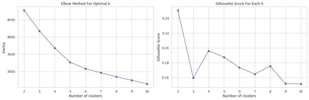
plt.figure(figsize=(15,5))

plt.subplot(1, 2, 1)
plt.plot(k_range, inertia, marker='o')
plt.xlabel('Number of clusters')
plt.ylabel('Inertia')
plt.title('Elbow Method For Optimal k')

plt.subplot(1, 2, 2)
plt.plot(k_range, silhouette_scores, marker='o')
plt.xlabel('Number of clusters')
plt.ylabel('Silhouette Score')
plt.title('Silhouette Score For Each k')

plt.tight_layout()
plt.show()

1.左图为肘部法则图，通过此图可以看到，在4和5的时候，曲线下降速率明显下降。
2.右图为轮廓系数图，在2时，轮廓系数最高，在4时也不错。
结合两个图，我们选择4作为聚类数，此时肘部法则图下降速率有明显下降，且是轮廓系数图中第二高的点。

7.2建立k均值聚类模型

In [20]:

# 执行K-均值聚类，选择4个聚类
kmeans_final = KMeans(n_clusters=4, random_state=15)
kmeans_final.fit(new_data)
# 获取聚类标签
cluster_labels = kmeans_final.labels_
# 将聚类标签添加到原始数据中以进行分析
data['Cluster'] = cluster_labels

7.3四类客户之间对比

7.3.1基本情况对比

In [21]:

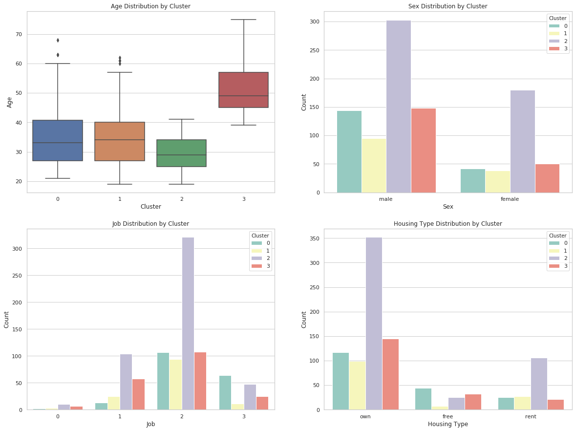
fig, axs = plt.subplots(2, 2, figsize=(20,15))

sns.boxplot(x='Cluster', y='Age', data=data, ax=axs[0, 0])
axs[0, 0].set_title('Age Distribution by Cluster')
axs[0, 0].set_xlabel('Cluster')
axs[0, 0].set_ylabel('Age')

sns.countplot(x='Sex', hue='Cluster', data=data, palette='Set3', ax=axs[0, 1])
axs[0, 1].set_title('Sex Distribution by Cluster')
axs[0, 1].set_xlabel('Sex')
axs[0, 1].set_ylabel('Count')

sns.countplot(x='Job', hue='Cluster', data=data, palette='Set3', ax=axs[1, 0])
axs[1, 0].set_title('Job Distribution by Cluster')
axs[1, 0].set_xlabel('Job')
axs[1, 0].set_ylabel('Count')

sns.countplot(x='Housing', hue='Cluster', data=data, palette='Set3', ax=axs[1, 1])
axs[1, 1].set_title('Housing Type Distribution by Cluster')
axs[1, 1].set_xlabel('Housing Type')
axs[1, 1].set_ylabel('Count')

Out[21]:

Text(0, 0.5, 'Count')

7.3.2经济情况对比

In [22]:

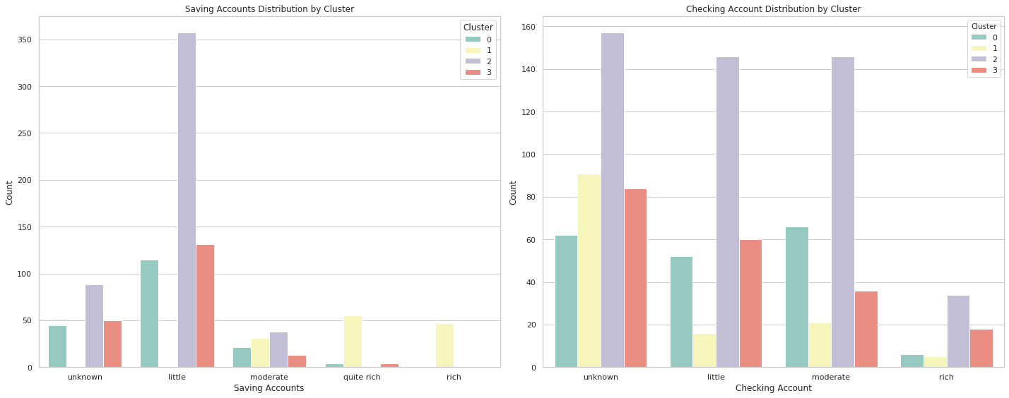
order_savings = ['unknown', 'little', 'moderate', 'quite rich', 'rich']
order_checking = ['unknown', 'little', 'moderate', 'rich']

fig, axs = plt.subplots(1, 2, figsize=(20,8))

sns.countplot(x='Saving accounts', hue='Cluster', data=data, order=order_savings, palette='Set3', ax=axs[0])
axs[0].set_title('Saving Accounts Distribution by Cluster')
axs[0].set_xlabel('Saving Accounts')
axs[0].set_ylabel('Count')
axs[0].legend(title='Cluster', loc='upper right')

sns.countplot(x='Checking account', hue='Cluster', data=data, order=order_checking, palette='Set3', ax=axs[1])
axs[1].set_title('Checking Account Distribution by Cluster')
axs[1].set_xlabel('Checking Account')
axs[1].set_ylabel('Count')

plt.tight_layout()
plt.show()

7.3.3贷款情况对比

In [23]:

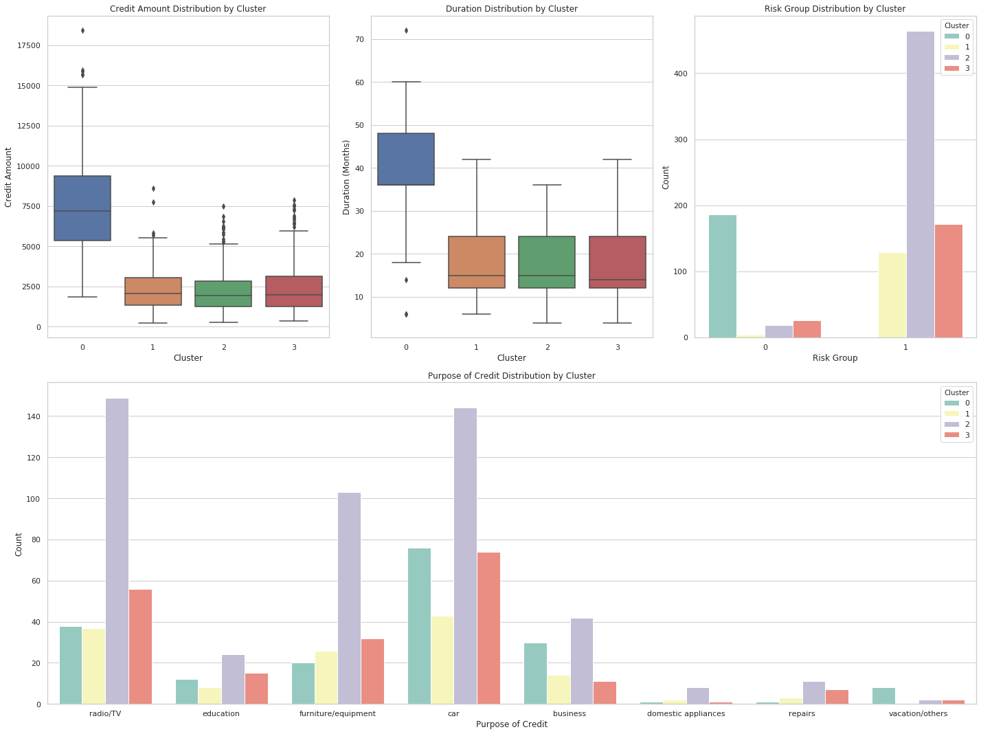
fig = plt.figure(figsize=(20,15))

# 创建2x2的图布局
ax1 = fig.add_subplot(2, 3, 1)
ax2 = fig.add_subplot(2, 3, 2)
ax3 = fig.add_subplot(2, 3, 3)
ax4 = fig.add_subplot(2, 1, 2)

sns.boxplot(x='Cluster', y='Credit amount', data=data, ax=ax1)
ax1.set_title('Credit Amount Distribution by Cluster')
ax1.set_xlabel('Cluster')
ax1.set_ylabel('Credit Amount')

sns.boxplot(x='Cluster', y='Duration', data=data, ax=ax2)
ax2.set_title('Duration Distribution by Cluster')
ax2.set_xlabel('Cluster')
ax2.set_ylabel('Duration (Months)')

sns.countplot(x='Risk Group', hue='Cluster', data=data, palette='Set3', ax=ax3)
ax3.set_title('Risk Group Distribution by Cluster')
ax3.set_xlabel('Risk Group')
ax3.set_ylabel('Count')

sns.countplot(x='Purpose', hue='Cluster', data=data, palette='Set3', ax=ax4)
ax4.set_title('Purpose of Credit Distribution by Cluster')
ax4.set_xlabel('Purpose of Credit')
ax4.set_ylabel('Count')

plt.tight_layout()
plt.show()

1.类型0（中高等额度需求，倾向于中长期贷款的高职业人群）:
用户画像：年龄主要在20-40岁之间，职业主要在2-3级，这一类人是住免租赁或者租房的占比远高于其他三类，储蓄账户状况主要集中在未知和少量，支票账户也是如此，主要集中在未知、少量和适中，贷款金额和贷款周期远超其他三类，贷款主要用于购车，根据风险评估，这类客户全部为高风险。
建议：银行和金融机构可以为这个群体提供中期汽车贷款产品，并且可以通过金融教育来提升他们的储蓄和投资能力。
2.类别1（较高储蓄能力，倾向于短期贷款的人群）:
用户画像：年龄分布比较均匀，与类型0相近，职业主要在2级，免租赁的占比较小，储蓄账户状况远超其他三类客户，贷款金额少，周期短，贷款主要用于购买设备，根据风险评估，这类客户全部为低风险。
建议：银行和金融机构可以为这个群体提供短期信用产品，同时考虑他们较高的储蓄能力，可以推广储蓄和投资相关产品。
3.类型2（短期贷款，储蓄能力有限的年轻化人群）:
用户画像：平均年龄在30岁以下，最大年龄不超过45岁，比其他三类都更年轻，职业主要集中在2级，但是其他等级都有存在，租房占比高于其他三类，蓄账户状况主要集中在未知和少量，支票账户主要集中在未知、少量和适中，这类客户的资金情况与类型0类似，贷款情况与类型1类似，风险评估绝大多数为低风险。
建议：鉴于他们是信用初建者和年轻消费者，银行和金融机构可以提供小额信用卡产品和财务规划服务。
4.类型3（短期贷款的高龄客户）:
用户画像：大龄客户，职业集中在1-2级，大部分有自己的房子，少部分是免租赁，蓄账户状况主要集中在未知和少量，支票账户每个等级均有占比，贷款情况与类型1和类型2类似，也是贷款金额少，周期短，同样的风险评估大多数是低风险。
建议：针对这类客户，银行和金融机构可以提供针对成熟消费者的产品和服务，如退休规划和健康保险，同时关注其稳定的信贷需求。

8.随机森林模型

通过构建用户画像后，可以认为客户贷款风险评估得到的结果是比较正确的，因此可以建立随机森林模型来预测客户是否存在高风险，以及探究哪个特征是划分风险的重要因素。

8.1数据处理

In [24]:

x = new_data
y = data['Risk Group']
#采用分层抽样来保证训练集和测试集中目标值与整体数据集的分布相似
x_train, x_test, y_train, y_test = train_test_split(x, y, test_size=0.3, random_state=10, stratify=y) #37分

In [25]:

#分离少数类和多数类
x_minority = x_train[y_train == 0]
y_minority = y_train[y_train == 0]
x_majority = x_train[y_train == 1]
y_majority = y_train[y_train == 1]
x_minority_resampled = resample(x_minority, replace=True, n_samples=len(x_majority), random_state=15)
y_minority_resampled = resample(y_minority, replace=True, n_samples=len(y_majority), random_state=15)
new_x_train = pd.concat([x_majority, x_minority_resampled])
new_y_train = pd.concat([y_majority, y_minority_resampled])

In [26]:

is_in_train = x_train.apply(lambda row: row.isin(new_x_train).all(), axis=1)
duplicates_in_test = x_train[is_in_train]

print(f"测试集中包含训练集的行数: {duplicates_in_test.shape[0]}")

测试集中包含训练集的行数: 0

8.2建立模型

In [27]:

rf_clf = RandomForestClassifier(random_state=15)
rf_clf.fit(new_x_train, new_y_train)

/opt/conda/lib/python3.6/site-packages/sklearn/ensemble/forest.py:245: FutureWarning: The default value of n_estimators will change from 10 in version 0.20 to 100 in 0.22.
  "10 in version 0.20 to 100 in 0.22.", FutureWarning)

Out[27]:

RandomForestClassifier(bootstrap=True, class_weight=None, criterion='gini',
                       max_depth=None, max_features='auto', max_leaf_nodes=None,
                       min_impurity_decrease=0.0, min_impurity_split=None,
                       min_samples_leaf=1, min_samples_split=2,
                       min_weight_fraction_leaf=0.0, n_estimators=10,
                       n_jobs=None, oob_score=False, random_state=15, verbose=0,
                       warm_start=False)

8.3模型评估

In [28]:

y_pred_rf = rf_clf.predict(x_test)
class_report_rf = classification_report(y_test, y_pred_rf)
print(class_report_rf)

              precision    recall  f1-score   support

           0       0.92      0.97      0.94        70
           1       0.99      0.97      0.98       230

    accuracy                           0.97       300
   macro avg       0.96      0.97      0.96       300
weighted avg       0.97      0.97      0.97       300

In [29]:

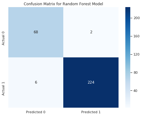
#绘制混淆矩阵
cm_rf = confusion_matrix(y_test, y_pred_rf)

plt.figure(figsize=(8, 6))
sns.heatmap(cm_rf, annot=True, fmt='g', cmap='Blues', 
            xticklabels=['Predicted 0', 'Predicted 1'], 
            yticklabels=['Actual 0', 'Actual 1'])
plt.title('Confusion Matrix for Random Forest Model')
plt.show()

模型评分如下:
1.精确度: 对于类别0，精确度为0.92，对于类别1，精确度为0.99。
2.召回率: 对于类别0，召回率为0.97，对于类别1，召回率为0.97。
3.F1得分: 对于类别0，F1得分为0.94，对于类别1，F1得分为0.98。
4.准确率: 0.97。
这是相当高的评价，可惜的就是数据中并没有包含客户贷款风险性这个特征，这个特征是通过聚类划分出来的，可能与实际有偏差，我们进一步探究哪个因素是划分的重要依据。

8.4模型重要特征度

In [30]:

rf_feature_importance = rf_clf.feature_importances_
feature_names = new_x_train.columns
rf_feature_df = pd.DataFrame({
    'Feature': feature_names,
    'Importance': rf_feature_importance
})
sorted_rf_feature_df = rf_feature_df.sort_values(by='Importance', ascending=False).head() #筛选出前五的重要特征

sorted_rf_feature_df

Out[30]:

	Feature	Importance
7	Duration	0.434162
6	Credit amount	0.385503
2	Job	0.058068
3	Housing	0.038544
0	Age	0.037094

可以看出来，聚类划分高风险和低风险主要取决于贷款金额和贷款期限。

9.结论

本项目通过可视化分析对数据进行初步探索，并利用聚类分析将客户分为不同的风险群体，由于数据集中缺乏直接的客户贷款风险标签，我们无法直接评估风险分类的准确性，因此，再次采用聚类分析（不考虑客户贷款风险特征），将数据分为四个类别，分别描述如下：
类0：中高等额度需求和中长期贷款倾向的高职业人群，被认为是高风险群体。
类1：具有较高储蓄能力和短期贷款倾向的客户，属于低风险群体。
类2：年轻群体，倾向于短期贷款且储蓄能力有限，为低风险群体。
类3：高龄客户，偏好短期贷款，也是低风险群体。
可以发现，分类结果与实际相符，可以构建随机森林模型来识别风险分类的关键因素。分析结果显示，贷款金额和贷款期限是划分风险的主要依据。虽然无法准确评估模型的精度，但该模型仍可作为初步风险评估的有效工具，从而提高风险识别的效率。