PRUNING FILTERS FOR EFFICIENT CONVNETS(L1)

论文地址：https://arxiv.org/abs/1608.08710

ABSTRACT

The success of CNNs in various applications is accompanied by a significant increase in the computation and parameter storage costs. Recent efforts toward reducing these overheads involve pruning and compressing the weights of various layers without hurting original accuracy. However, magnitude-based pruning of weights reduces a significant number of parameters from the fully connected layers and may not adequately reduce the computation costs in the convolutional layers due to irregular sparsity in the pruned networks. We present an acceleration method for CNNs, where we prune filters from CNNs that are identified as having a small effect on the output accuracy. By removing whole filters in the network together with their connecting feature maps, the computation costs are reduced significantly. In contrast to pruning weights, this approach does not result in sparse connectivity patterns. Hence, it does not need the support of sparse convolution libraries and can work with existing efficient BLAS libraries for dense matrix multiplications. We show that even simple filter pruning techniques can reduce inference costs for
VGG-16 by up to 34% and ResNet-110 by up to 38% on CIFAR10 while regaining close to the original accuracy by retraining the networks.

摘要

CNN 在各种应用中的成功伴随着计算和参数存储成本的显着增加。最近为减少这些开销所做的努力包括在不损害原始准确性的情况下修剪和压缩各个层的权重。然而，基于幅度的权重剪枝减少了来自全连接层的大量参数，并且由于剪枝网络中的不规则稀疏性，可能无法充分降低卷积层中的计算成本。我们提出了一种 CNN 加速方法，其中我们从 CNN 中修剪那些被认为对输出精度影响较小的滤波器。通过删除网络中的整个过滤器及其连接的特征图，计算成本显着降低。与修剪权重相比，这种方法不会导致稀疏连接模式。因此，它不需要稀疏卷积库的支持，并且可以与现有的高效 BLAS 库一起进行密集矩阵乘法。我们证明，即使是简单的过滤器修剪技术也可以在 CIFAR10 上将 VGG-16 的推理成本降低高达 34%，将 ResNet-110 的推理成本降低高达 38%，同时通过重新训练网络来恢复接近原始的精度。

1 INTRODUCTION（简介）

The ImageNet challenge has led to significant advancements in exploring various architectural
choices in CNNs (Russakovsky et al. (2015); Krizhevsky et al. (2012); Simonyan & Zisserman
(2015); Szegedy et al. (2015a); He et al. (2016)). The general trend since the past few years has
been that the networks have grown deeper, with an overall increase in the number of parameters and convolution operations. These high capacity networks have significant inference costs especially when used with embedded sensors or mobile devices where computational and power resources may be limited. For these applications, in addition to accuracy, computational efficiency and small network sizes are crucial enabling factors (Szegedy et al. (2015b)). In addition, for web services that provide image search and image classification APIs that operate on a time budget often serving hundreds of thousands of images per second, benefit significantly from lower inference times.

ImageNet 挑战在探索 CNN 的各种架构选择方面取得了重大进展（Russakovsky 等人 (2015)；Krizhevsky 等人 (2012)；Simonyan & Zisserman (2015)；Szegedy 等人 (2015a)；He等人（2016））。过去几年来的总体趋势是网络变得更深，参数数量和卷积运算的数量总体增加。这些高容量网络具有显着的推理成本，特别是当与计算和电力资源可能有限的嵌入式传感器或移动设备一起使用时。对于这些应用程序，除了准确性之外，计算效率和小网络规模也是至关重要的促成因素（Szegedy 等人（2015b））。此外，对于提供图像搜索和图像分类 API 的 Web 服务来说，这些 API 在时间预算上运行，通常每秒提供数十万张图像，因此可以从较短的推理时间中获益匪浅。

There has been a significant amount of work on reducing the storage and computation costs by model compression (Le Cun et al. (1989); Hassibi & Stork (1993); Srinivas & Babu (2015); Han et al. (2015); Mariet & Sra (2016)). Recently Han et al. (2015; 2016b) report impressive compression rates on AlexNet (Krizhevsky et al. (2012)) and VGGNet (Simonyan & Zisserman (2015)) by pruning weights with small magnitudes and then retraining without hurting the overall accuracy. However, pruning parameters does not necessarily reduce the computation time since the majority of the parameters removed are from the fully connected layers where the computation cost is low, e.g., the fully connected layers of VGG-16 occupy 90% of the total parameters but only contribute less than 1% of the overall floating point operations (FLOP). They also demonstrate that the convolutional layers can be compressed and accelerated (Iandola et al. (2016)), but additionally require sparse BLAS libraries or even specialized hardware (Han et al. (2016a)). Modern libraries that provide speedup using sparse operations over CNNs are often limited (Szegedy et al. (2015a); Liu et al. (2015)) and maintaining sparse data structures also creates an additional storage overhead which can be significant for low-precision weights.

在通过模型降低存储和计算成本方面已经做了大量的工作 压缩（Le Cun 等人 (1989)；Hassibi & Stork (1993)；Srinivas & Babu (2015)；Han 等人。 （2015）；玛丽特和斯拉（2016））。最近韩等人。 （2015；2016b）报告了令人印象深刻的压缩率 在 AlexNet (Krizhevsky et al. (2012)) 和 VGGNet (Simonyan & Zisserman (2015)) 上通过剪枝 小幅度的权重，然后在不损害整体准确性的情况下重新训练。然而， 修剪参数并不一定会减少计算时间，因为大多数 删除的参数来自计算成本较低的全连接层，例如 VGG-16 的全连接层占据了总参数的 90%，但只贡献了不到 占整体浮点运算 (FLOP) 的 1%。他们还证明了卷积 层可以被压缩和加速（Iandola 等人（2016）），但还需要稀疏的 BLAS 库甚至专门的硬件（Han 等人（2016a））。在 CNN 上使用稀疏操作提供加速的现代库通常是有限的（Szegedy 等人（2015a）；Liu 等人（2015）），并且维护稀疏数据结构也会产生额外的存储开销，这对于低精度权重来说可能非常重要。

Recent work on CNNs have yielded deep architectures with more efficient design (Szegedy et al.
(2015a;b); He & Sun (2015); He et al. (2016)), in which the fully connected layers are replaced with average pooling layers (Lin et al. (2013); He et al. (2016)), which reduces the number of parameters significantly. The computation cost is also reduced by downsampling the image at an early stage to reduce the size of feature maps (He & Sun (2015)). Nevertheless, as the networks continue to become deeper, the computation costs of convolutional layers continue to dominate.

最近关于 CNN 的工作已经产生了具有更高效设计的深层架构（Szegedy 等人（2015a；b）；He & Sun（2015）；He 等人（2016）），其中全连接层被平均池化取代层（Lin et al. (2013); He et al. (2016)），这显着减少了参数的数量。通过在早期阶段对图像进行下采样以减小特征图的大小，还可以降低计算成本（He & Sun (2015)）。然而，随着网络继续变得更深，卷积层的计算成本继续占据主导地位。

CNNs with large capacity usually have significant redundancy among different filters and feature
channels. In this work, we focus on reducing the computation cost of well-trained CNNs by pruning filters. Compared to pruning weights across the network, filter pruning is a naturally structured way of pruning without introducing sparsity and therefore does not require using sparse libraries or any specialized hardware. The number of pruned filters correlates directly with acceleration by reducing the number of matrix multiplications, which is easy to tune for a target speedup. In addition, instead of layer-wise iterative fine-tuning (retraining), we adopt a one-shot pruning and retraining strategy to save retraining time for pruning filters across multiple layers, which is critical for pruning very deep networks. Finally, we observe that even for ResNets, which have significantly fewer parameters and inference costs than AlexNet or VGGNet, still have about 30% of FLOP reduction without sacrificing too much accuracy. We conduct sensitivity analysis for convolutional layers in ResNets that improves the understanding of ResNets.

大容量的 CNN 通常在不同的滤波器和特征通道之间具有显着的冗余。在这项工作中，我们专注于通过修剪过滤器来降低训练有素的 CNN 的计算成本。与整个网络的剪枝权重相比，过滤器剪枝是一种自然结构化的剪枝方式，不会引入稀疏性，因此不需要使用稀疏库或任何专门的硬件。修剪滤波器的数量通过减少矩阵乘法的数量与加速直接相关，这很容易调整以实现目标加速。此外，我们不采用逐层迭代微调（重新训练），而是采用一次性剪枝和重新训练策略来节省跨多层剪枝滤波器的重新训练时间，这对于剪枝非常深的网络至关重要。最后，我们观察到，即使对于参数和推理成本明显少于 AlexNet 或 VGGNet 的 ResNet，仍然可以减少约 30% 的 FLOP，而不会牺牲太多的准确性。我们对 ResNet 中的卷积层进行敏感性分析，以提高对 ResNet 的理解。

2 RELATED WORK（相关工作）

The early work by Le Cun et al. (1989) introduces Optimal Brain Damage, which prunes weights
with a theoretically justified saliency measure. Later, Hassibi & Stork (1993) propose Optimal Brain Surgeon to remove unimportant weights determined by the second-order derivative information. Mariet & Sra (2016) reduce the network redundancy by identifying a subset of diverse neurons that does not require retraining. However, this method only operates on the fully-connected layers and introduce sparse connections.

Le Cun 等人的早期工作。 (1989) 引入了最佳脑损伤，它通过理论上合理的显着性度量来修剪权重。后来，Hassibi & Stork (1993) 提出了 Optimal Brain Surgeon 来去除由二阶导数信息确定的不重要权重。 Mariet & Sra (2016) 通过识别不需要重新训练的不同神经元子集来减少网络冗余。然而，该方法仅在全连接层上运行并引入稀疏连接。

To reduce the computation costs of the convolutional layers, past work have proposed to approximate convolutional operations by representing the weight matrix as a low rank product of two smaller matrices without changing the original number of filters (Denil et al. (2013); Jaderberg et al. (2014); Zhang et al. (2015b;a); Tai et al. (2016); Ioannou et al. (2016)). Other approaches to reduce the convolutional overheads include using FFT based convolutions (Mathieu et al. (2013)) and fast convolution using the Winograd algorithm (Lavin & Gray (2016)). Additionally, quantization (Han et al. (2016b)) and binarization (Rastegari et al. (2016); Courbariaux & Bengio (2016)) can be used to reduce the model size and lower the computation overheads. Our method can be used in addition to these techniques to reduce computation costs without incurring additional overheads.

为了减少卷积层的计算成本，过去的工作提出通过将权重矩阵表示为两个较小矩阵的低秩乘积来近似卷积运算，而不改变滤波器的原始数量（Denil 等人（2013）；Jaderberg 等人）等人(2014）；Zhang 等人（2015b；a）；Tai 等人（2016）；Ioannou 等人（2016))。减少卷积开销的其他方法包括使用基于 FFT 的卷积（Mathieu et al. (2013)）和使用 Winograd 算法的快速卷积（Lavin & Gray (2016)）。此外，量化（Han et al. (2016b)）和二值化（Rastegari et al. (2016)；Courbariaux & Bengio (2016)）可用于减小模型大小并降低计算开销。除了这些技术之外，还可以使用我们的方法来降低计算成本，而不会产生额外的开销。

Several work have studied removing redundant feature maps from a well trained network (Anwar et al. (2015); Polyak &Wolf (2015)). Anwar et al. (2015) introduce a three-level pruning of the weights and locate the pruning candidates using particle filtering, which selects the best combination from a number of random generated masks. Polyak & Wolf (2015) detect the less frequently activated feature maps with sample input data for face detection applications. We choose to analyze the filter weights and prune filters with their corresponding feature maps using a simple magnitude based measure, without examining possible combinations. We also introduce network-wide holistic approaches to prune filters for simple and complex convolutional network architectures.

有几项工作研究了从训练有素的网络中删除冗余特征图（Anwar 等人 (2015)；Polyak &Wolf (2015)）。安瓦尔等人。 (2015)引入了权重的三级修剪，并使用粒子过滤来定位修剪候选者，粒子过滤从许多随机生成的掩模中选择最佳组合。 Polyak & Wolf (2015) 使用人脸检测应用的样本输入数据来检测不太频繁激活的特征图。我们选择使用简单的基于幅度的测量来分析滤波器权重和修剪滤波器及其相应的特征图，而不检查可能的组合。我们还引入了网络范围的整体方法来修剪简单和复杂的卷积网络架构的滤波器。

Concurrently with our work, there is a growing interest in training compact CNNs with sparse constraints (Lebedev & Lempitsky (2016); Zhou et al. (2016); Wen et al. (2016)). Lebedev & Lempitsky (2016) leverage group-sparsity on the convolutional filters to achieve structured brain damage, i.e., prune the entries of the convolution kernel in a group-wise fashion. Zhou et al. (2016) add group-sparse regularization on neurons during training to learn compact CNNs with reduced filters. Wen et al. (2016) add structured sparsity regularizer on each layer to reduce trivial filters, channels or even layers. In the filter-level pruning, all above work use 2,1-norm as a regularizer. Similar to the above work, we use 1-norm to select unimportant filters and physically prune them. Our fine-tuning process is the same as the conventional training procedure, without introducing additional regularization. Our approach does not introduce extra layer-wise meta-parameters for the regularizer except for the percentage of filters to be pruned, which is directly related to the desired speedup. By employing stage-wise pruning, we can set a single pruning rate for all layers in one stage.

在我们工作的同时，人们对训练稀疏的紧凑型 CNN 越来越感兴趣 约束（Lebedev & Lempitsky (2016)；Zhou et al. (2016)；Wen et al. (2016)）。Lebedev& Lempitsky (2016) 利用卷积滤波器的组稀疏性来实现结构化大脑 损坏，即以分组方式修剪卷积核的条目。周等人。 (2016) 在训练过程中对神经元添加组稀疏正则化，以减少学习紧凑型 CNN 过滤器。文等人。 (2016) 在每一层上添加结构化稀疏正则化器以减少琐碎的过滤器， 通道甚至层。在滤波器级剪枝中，上述工作均使用 l2,1-范数作为正则化器。与上述工作类似，我们使用 l1-norm 来选择不重要的过滤器并对其进行物理修剪。我们的微调过程与传统的训练过程相同，没有引入额外的正则化。我们的方法不会为正则化器引入额外的分层元参数，除了要修剪的滤波器的百分比之外，这与所需的加速直接相关。通过采用阶段式剪枝，我们可以在一个阶段为所有层设置单一剪枝率。

3 PRUNING FILTERS AND FEATURE MAPS(剪枝过滤器和特征图)

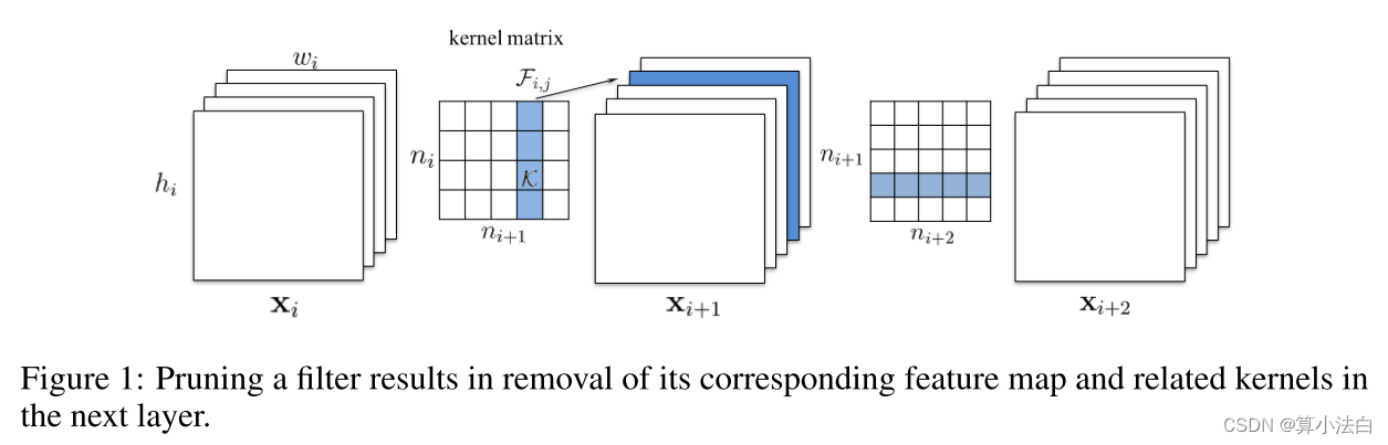
图 1：修剪过滤器会导致删除下一层中相应的特征图和相关内核。

令 ni 表示第 i 个卷积层的输入通道数，hi/wi 表示输入特征图的高度/宽度。卷积层将输入特征图 xi ∈ Rni×hi×wi 转换为输出特征图 xi+1 ∈ Rni+1×hi+1×wi+1 ，用作下一个卷积层的输入特征图。这是通过在 ni 个输入通道上应用 ni+1 个 3D 滤波器 Fi,j ∈ Rni×k×k 来实现的，其中一个滤波器生成一个特征图。每个滤波器由 ni 个 2D 内核 K ∈ Rk×k（例如 3 × 3）组成。所有滤波器共同构成了核矩阵 Fi ∈ Rni×ni+1×k×k。卷积层的运算次数为ni+1nik2hi+1wi+1。如图1所示，当过滤器Fi,j被剪枝时，其对应的特征图xi+1,j被移除，从而减少了nik2hi+1wi+1操作。应用到从下一个卷积层的滤波器移除的特征图上的内核也被移除，这节省了额外的 ni+2k2hi+2wi+2 操作。修剪第 i 层的 m 个滤波器将减少第 i 层和第 i+1 层的 m/ni+1 计算成本。

3.1 DETERMINING WHICH FILTERS TO PRUNE WITHIN A SINGLE LAYER(3.1 确定单层内要修剪哪些过滤器)

我们的方法从训练有素的模型中删除不太有用的过滤器，以提高计算效率，同时最大限度地减少准确性下降。我们通过计算滤波器的绝对权重  |Fi,j | 之和来衡量每层滤波器的相对重要性，即其 1-范数 Fi,j1。由于输入通道的数量 ni 在滤波器之间是相同的，  |Fi,j |也表示其核权重的平均大小。该值给出了输出特征图大小的期望。与该层中的其他过滤器相比，具有较小内核权重的过滤器往往会产生激活较弱的特征图。图 2(a) 说明了在 CIFAR-10 数据集上训练的 VGG-16 网络中每个卷积层的滤波器绝对权重总和的分布，其中各层的分布差异很大。我们发现，与修剪相同数量的随机或最大过滤器相比，修剪最小过滤器效果更好（第 4.4 节）。与基于激活的特征图修剪的其他标准（第 4.5 节）相比，我们发现l1-范数是无数据滤波器选择的良好标准。

The procedure of pruning m filters from the ith convolutional layer is as follows:
1. For each filter Fi,j , calculate the sum of its absolute kernel weights
2. Sort the filters by sj.
3. Prune m filters with the smallest sum values and their corresponding feature maps. The
kernels in the next convolutional layer corresponding to the pruned feature maps are also
removed.
4. A new kernel matrix is created for both the ith and i + 1th layers, and the remaining kernel
weights are copied to the new model.

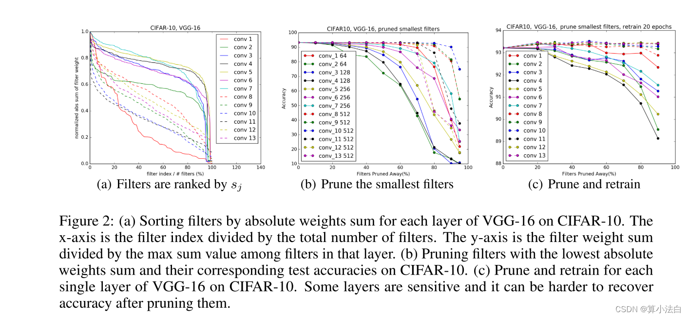
图 2：(a) 按 CIFAR-10 上 VGG-16 每层的绝对权重总和对过滤器进行排序。 x 轴是过滤器索引除以过滤器总数。 y 轴是滤波器权重总和除以该层滤波器之间的最大总和值。 (b) 具有最低绝对权重和的剪枝滤波器及其在 CIFAR-10 上的相应测试精度。 (c) 在 CIFAR-10 上修剪和重新训练 VGG-16 的每个单层。有些层很敏感，修剪它们后很难恢复准确性。

从第 i 个卷积层剪枝 m 个滤波器的过程如下：

1. 对于每个滤波器 Fi,j ，计算其绝对核权重之和 sj = ni l=1  |Kl|。

2. 按 sj 对过滤器进行排序。

3. 剪枝具有最小和值的 m 个滤波器及其对应的特征图。与修剪后的特征图相对应的下一个卷积层中的内核也被删除。

4. 为第 i 层和第 i+1 层创建一个新的核矩阵，并将剩余的核权重复制到新模型中。

Relationship to pruning weights Pruning filters with low absolute weights sum is similar to pruning
low magnitude weights (Han et al. (2015)). Magnitude-based weight pruning may prune away whole filters when all the kernel weights of a filter are lower than a given threshold. However, it requires a careful tuning of the threshold and it is difficult to predict the exact number of filters that will eventually be pruned. Furthermore, it generates sparse convolutional kernels which can be hard to accelerate given the lack of efficient sparse libraries, especially for the case of low-sparsity.

与剪枝权重的关系 具有低绝对权重总和的剪枝滤波器与剪枝低幅值权重类似（Han 等(2015))。当过滤器的所有内核权重低于给定阈值时，基于幅度的权重修剪可以修剪掉整个过滤器。然而，它需要仔细调整阈值，并且很难预测最终将被修剪的过滤器的确切数量。此外，它生成稀疏卷积核，由于缺乏有效的稀疏库，特别是在低稀疏性的情况下，很难加速。

与滤波器上的群稀疏正则化的关系最近的工作（Zhou et al. (2016); Wen et al. (2016)）应用群稀疏正则化（ ||Fi,j||2 或 l2,1-范数）在卷积滤波器上，这也有利于具有小 l2-范数的归零滤波器，即 Fi,j = 0。在实践中，我们没有观察到滤波器的 l2-范数和 l1-范数之间存在明显差异选择，因为重要的过滤器往往对这两种度量都有很大的值（附录 6.1）。在训练过程中将多个过滤器的权重清零与使用 3.4 节中介绍的迭代剪枝和再训练策略剪枝过滤器具有类似的效果。

3.2 确定单层对剪枝的敏感性

为了了解每一层的敏感性，我们独立地剪枝每一层并评估所得剪枝网络在验证集上的准确性。图 2(b) 显示，当过滤器被修剪掉时，保持其准确性的层对应于图 2(a) 中具有较大斜率的层。相反，坡度相对平坦的层对修剪更为敏感。我们根据修剪的敏感性凭经验确定每层要修剪的过滤器数量。对于 VGG-16 或 ResNets 等深度网络，我们观察到同一阶段的层（具有相同的特征图大小）对剪枝具有相似的敏感性。为了避免引入逐层元参数，我们对同一阶段的所有层使用相同的剪枝率。对于对修剪敏感的层，我们修剪这些层的较小比例或完全跳过修剪它们。

3.3 跨多层修剪过滤器

我们现在讨论如何跨网络修剪过滤器。之前的工作逐层修剪权重，然后迭代地重新训练并补偿任何准确性损失（Han et al. (2015)）。然而，了解如何同时修剪多个层的过滤器可能很有用：1) 对于深层网络，逐层修剪和重新训练可能非常耗时 2) 整个网络的修剪层可以提供整体视图网络的鲁棒性导致网络更小 3) 对于复杂的网络，可能需要采用整体方法。例如，对于 ResNet，修剪身份特征图或每个残差块的第二层会导致其他层的额外修剪。

To prune filters across multiple layers, we consider two strategies for layer-wise filter selection:

• Independent pruning determines which filters should be pruned at each layer independent of other layers.

• Greedy pruning accounts for the filters that have been removed in the previous layers. This strategy does not consider the kernels for the previously pruned feature maps while calculating the sum of absolute weights.

Figure 3 illustrates the difference between two approaches in calculating the sum of absolute weights. The greedy approach, though not globally optimal, is holistic and results in pruned networks with higher accuracy especially when many filters are pruned.

为了跨多个层修剪过滤器，我们考虑两种逐层过滤器选择策略：

• 独立修剪确定应在每一层独立于其他层修剪哪些过滤器。

• 贪婪修剪考虑了先前层中已删除的过滤器。该策略在计算绝对权重之和时不考虑先前修剪的特征图的内核。

图 3 说明了两种方法在计算绝对权重总和方面的差异。贪婪方法虽然不是全局最优的，但它是整体的，并且会导致修剪后的网络具有更高的准确度，尤其是在修剪许多过滤器时。

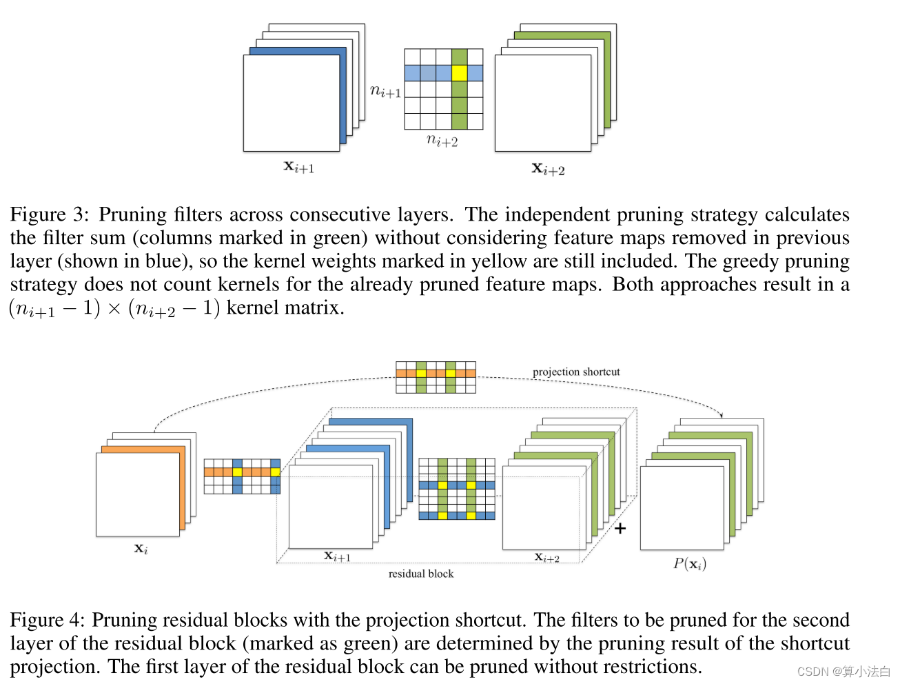
For simpler CNNs like VGGNet or AlexNet, we can easily prune any of the filters in any convolutional layer. However, for complex network architectures such as Residual networks (He et al. (2016)), pruning filters may not be straightforward. The architecture of ResNet imposes restrictions and the filters need to be pruned carefully. We show the filter pruning for residual blocks with projection mapping in Figure 4. Here, the filters of the first layer in the residual block can be arbitrarily pruned, as it does not change the number of output feature maps of the block. However, the correspondence between the output feature maps of the second convolutional layer and the identity feature maps makes it difficult to prune. Hence, to prune the second convolutional layer of the residual block, the corresponding projected feature maps must also be pruned. Since the identical feature maps are more important than the added residual maps, the feature maps to be pruned should be determined by the pruning results of the shortcut layer. To determine which identity feature maps are to be pruned, we use the same selection criterion based on the filters of the shortcut convolutional layers (with 1 × 1 kernels). The second layer of the residual block is pruned with the same filter index as selected by the pruning of the shortcut layer.

对于像 VGGNet 或 AlexNet 这样更简单的 CNN，我们可以轻松地修剪任何卷积层中的任何过滤器。然而，对于残差网络（He et al. (2016)）等复杂的网络架构，修剪过滤器可能并不简单。 ResNet 的架构施加了限制，需要仔细修剪过滤器。我们在图4中展示了使用投影映射对残差块进行滤波器剪枝。这里，残差块中第一层的滤波器可以任意剪枝，因为它不会改变块的输出特征图的数量。然而，第二个卷积层的输出特征图和身份特征图之间的对应关系使得修剪变得困难。因此，为了修剪残差块的第二个卷积层，还必须修剪相应的投影特征图。由于相同的特征图比添加的残差图更重要，因此要修剪的特征图应由快捷层的修剪结果确定。为了确定要修剪哪些身份特征图，我们使用基于快捷卷积层（具有 1 × 1 内核）的滤波器的相同选择标准。使用与快捷层的修剪所选择的相同的滤波器索引来修剪残差块的第二层。

3.4 RETRAINING PRUNED NETWORKS TO REGAIN ACCURACY（重新训练修剪后的网络以恢复准确性）

After pruning the filters, the performance degradation should be compensated by retraining the
network. There are two strategies to prune the filters across multiple layers:

1. Prune once and retrain: Prune filters of multiple layers at once and retrain them until the original accuracy is restored.
2. Prune and retrain iteratively: Prune filters layer by layer or filter by filter and then retrain iteratively. The model is retrained before pruning the next layer for the weights to adapt to the changes from the pruning process.

We find that for the layers that are resilient to pruning, the prune and retrain once strategy can be used to prune away significant portions of the network and any loss in accuracy can be regained by retraining for a short period of time (less than the original training time). However, when some filters from the sensitive layers are pruned away or large portions of the networks are pruned away, it may not be possible to recover the original accuracy. Iterative pruning and retraining may yield better results, but the iterative process requires many more epochs especially for very deep networks.

修剪过滤器后，应通过重新训练网络来补偿性能下降。跨多个层的过滤器剪枝有两种策略：

1. 剪枝一次并重新训练：一次剪枝多个层的过滤器并重新训练它们，直到恢复原始精度。

2. 迭代修剪和重新训练：逐层修剪过滤器或逐个过滤器过滤，然后迭代重新训练。在修剪下一层权重之前，会重新训练模型，以适应修剪过程中的变化。

我们发现，对于对剪枝有弹性的层，可以使用剪枝和重新训练一次策略来剪掉网络的重要部分，并且可以通过短时间的重新训练（小于原始时间）来恢复任何准确性损失。训练时间）。然而，当敏感层的一些过滤器被剪掉或网络的大部分被剪掉时，可能无法恢复原始的精度。迭代剪枝和重新训练可能会产生更好的结果，但迭代过程需要更多的时期，尤其是对于非常深的网络。

4 EXPERIMENTS（实验）

我们修剪了两种类型的网络：简单 CNN（CIFAR-10 上的 VGG-16）和残差网络（CIFAR-10 上的 ResNet-56/110 和 ImageNet 上的 ResNet-34）。与经常用于演示模型压缩的 AlexNet 或 VGG（在 ImageNet 上）不同，VGG（在 CIFAR-10 上）和残差网络在全连接层中的参数较少。因此，从这些网络中修剪大部分参数具有挑战性。我们在 Torch7 中实现了过滤器修剪方法（Collobert 等人（2011））。修剪过滤器时，将创建一个具有较少过滤器的新模型，并将修改层的剩余参数以及未受影响的层复制到新模型中。此外，如果对卷积层进行剪枝，则后续批量归一化层的权重也会被删除。为了获得每个网络的基线精度，我们从头开始训练每个模型，并遵循与 ResNet 相同的预处理和超参数（He et al. (2016)）。对于重新训练，我们使用恒定学习率 0.001，对 CIFAR-10 重新训练 40 个时期，对 ImageNet 重新训练 20 个时期，这相当于原始训练时期的四分之一。过去的工作报告了高达 3 倍的原始训练时间来重新训练修剪后的网络（Han 等人（2015））。

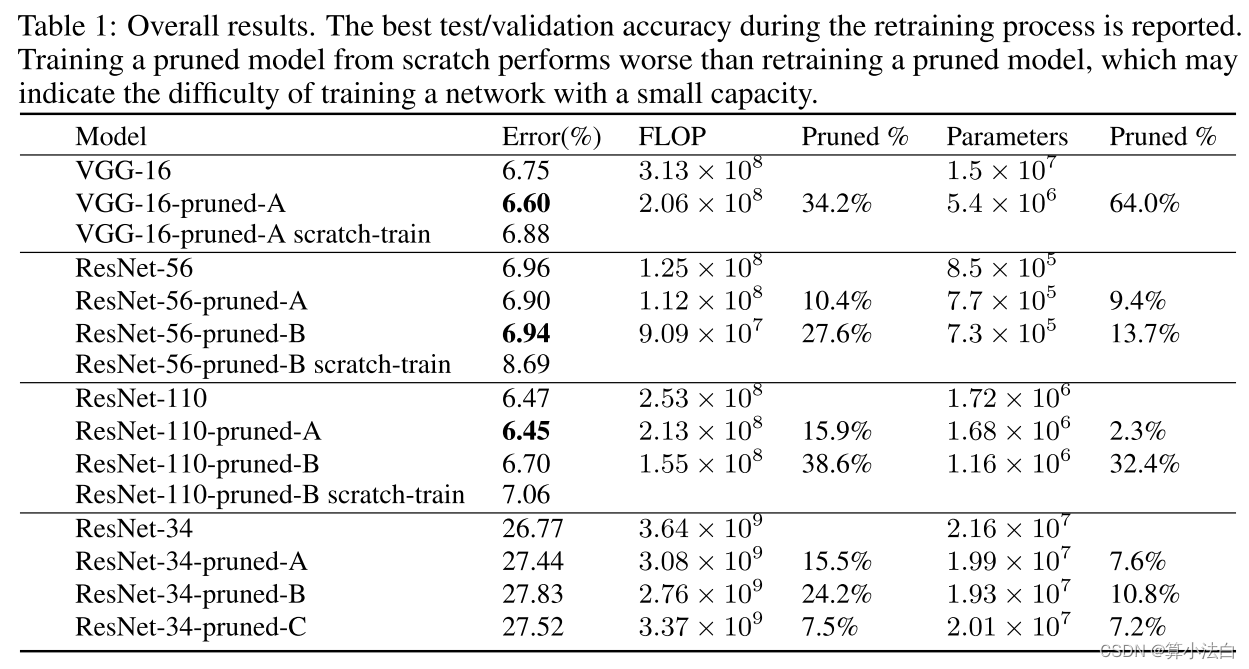
表 1：总体结果。报告再训练过程中的最佳测试/验证准确性。从头开始训练剪枝模型比重新训练剪枝模型表现更差，这可能表明训练小容量网络的难度。

4.1 VGG-16 ON CIFAR-10

VGG-16 is a high-capacity network originally designed for the ImageNet dataset (Simonyan &
Zisserman (2015)). Recently, Zagoruyko (2015) applies a slightly modified version of the model
on CIFAR-10 and achieves state of the art results. As shown in Table 2, VGG-16 on CIFAR-10
consists of 13 convolutional layers and 2 fully connected layers, in which the fully connected layers do not occupy large portions of parameters due to the small input size and less hidden units. We use the model described in Zagoruyko (2015) but add Batch Normalization (Ioffe & Szegedy (2015)) layer after each convolutional layer and the first linear layer, without using Dropout (Srivastava et al. (2014)). Note that when the last convolutional layer is pruned, the input to the linear layer is changed and the connections are also removed.

表 2：CIFAR-10 上的 VGG-16 和剪枝模型。最后两列显示了特征映射的数量以及修剪模型中 FLOP 减少的百分比。

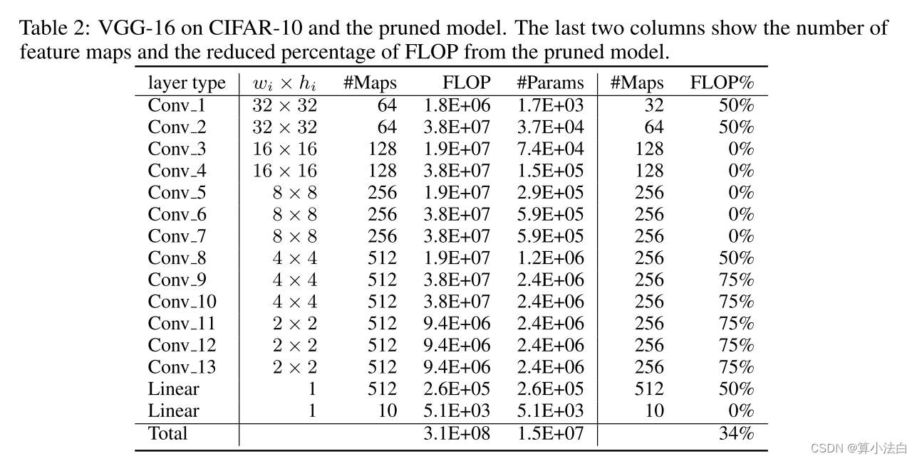
VGG-16 是最初为 ImageNet 数据集设计的高容量网络（Simonyan & Zisserman (2015)）。最近，Zagoruyko（2015）在 CIFAR-10 上应用了该模型的稍微修改版本，并取得了最先进的结果。如表2所示，CIFAR-10上的VGG-16由13个卷积层和2个全连接层组成，其中全连接层由于输入尺寸小且隐藏单元较少而不会占用大部分参数。我们使用 Zagoruyko (2015) 中描述的模型，但在每个卷积层和第一个线性层之后添加批量归一化 (Ioffe & Szegedy (2015)) 层，而不使用 Dropout (Srivastava et al.(2014))。请注意，当最后一个卷积层被修剪时，线性层的输入会发生变化，并且连接也会被删除。

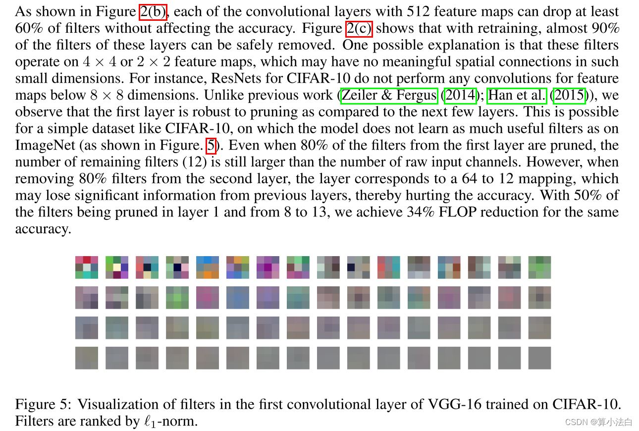
图 5：在 CIFAR-10 上训练的 VGG-16 第一个卷积层中的滤波器的可视化。过滤器按 l1-范数排序。

如图 2(b) 所示，每个具有 512 个特征图的卷积层可以在不影响精度的情况下丢弃至少 60% 的滤波器。图 2(c) 显示，通过重新训练，这些层中几乎 90% 的过滤器都可以被安全地移除。一种可能的解释是，这些滤波器在 4 × 4 或 2 × 2 特征图上运行，这些特征图在如此小的维度中可能没有有意义的空间连接。例如，CIFAR-10 的 ResNet 不会对低于 8 × 8 维度的特征图执行任何卷积。与之前的工作（Zeiler & Fergus (2014)；Han et al. (2015)）不同，我们观察到与接下来的几层相比，第一层对于修剪具有鲁棒性。对于像 CIFAR-10 这样的简单数据集，这是可能的，在该数据集上，模型不会像在 ImageNet 上那样学习那么多有用的过滤器（如图 5 所示）。即使第一层中 80% 的滤波器被修剪，剩余滤波器的数量 (12) 仍然大于原始输入通道的数量。然而，当从第二层中删除 80% 的滤波器时，该层对应于 64 到 12 的映射，这可能会丢失先前层的重要信息，从而损害准确性。通过在第 1 层和第 8 层到第 13 层修剪 50% 的滤波器，我们在相同的精度下实现了 34% 的 FLOP 减少。

4.2 RESNET-56/110 ON CIFAR-10

ResNets for CIFAR-10 have three stages of residual blocks for feature maps with sizes of 32 × 32,16 × 16 and 8 × 8. Each stage has the same number of residual blocks. When the number of feature maps increases, the shortcut layer provides an identity mapping with an additional zero padding for the increased dimensions. Since there is no projection mapping for choosing the identity feature maps, we only consider pruning the first layer of the residual block. As shown in Figure 6, most of the layers are robust to pruning. For ResNet-110, pruning some single layers without retraining even improves the performance. In addition, we find that layers that are sensitive to pruning (layers 20, 38 and 54 for ResNet-56, layer 36, 38 and 74 for ResNet-110) lie at the residual blocks close to the layers where the number of feature maps changes, e.g., the first and the last residual blocks for each stage. We believe this happens because the precise residual errors are necessary for the newly added empty feature maps.

CIFAR-10 的 ResNet 对于尺寸为 32 × 32 的特征图具有三级残差块， 16 × 16 和 8 × 8。每个阶段都有相同数量的残差块。当特征数量 映射增加，快捷方式层提供了带有附加零填充的恒等映射 增加的尺寸。由于没有用于选择身份特征的投影映射 映射时，我们只考虑修剪残差块的第一层。如图6所示，大部分 这些层对修剪具有鲁棒性。对于 ResNet-110，在不重新训练的情况下修剪一些单层甚至可以提高性能。此外，我们发现对剪枝敏感的层（ResNet-56 的层 20、38 和 54 ResNet-110 的层 36、38 和 74）位于靠近特征图数量的层的残差块处。变化，例如每个阶段的第一个和最后一个残差块。我们认为发生这种情况是因为新添加的空特征图需要精确的残差误差。

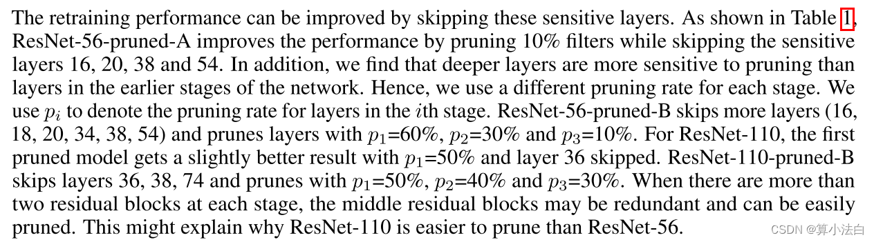
通过跳过这些敏感层可以提高重新训练性能。如表 1 所示，ResNet-56-pruned-A 通过修剪 10% 的滤波器，同时跳过敏感层 16、20、38 和 54 来提高性能。此外，我们发现更深的层比中的层对修剪更敏感。网络的早期阶段。因此，我们为每个阶段使用不同的剪枝率。我们用 pi 表示第 i 阶段各层的剪枝率。 ResNet-56-pruned-B 跳过更多层（16、18、20、34、38、54）并修剪 p1=60%、p2=30% 和 p3=10% 的层。对于 ResNet-110，第一个剪枝模型在 p1=50% 且跳过第 36 层时获得了稍好的结果。 ResNet-110-pruned-B 跳过第 36、38、74 层，并用 p1=50%、p2=40% 和 p3=30% 进行修剪。当每个阶段有两个以上的残差块时，中间的残差块可能是冗余的并且可以很容易地被修剪。这也许可以解释为什么 ResNet-110 比 ResNet-56 更容易修剪。

4.3 RESNET-34 ON ILSVRC2012

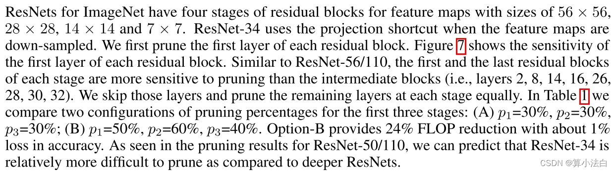
ImageNet 的 ResNet 对于尺寸为 56 × 56、28 × 28、14 × 14 和 7 × 7 的特征图有四个阶段的残差块。ResNet-34 在对特征图进行下采样时使用投影快捷方式。我们首先修剪每个残差块的第一层。图7显示了每个残差块的第一层的灵敏度。与 ResNet-56/110 类似，每个阶段的第一个和最后一个残差块比中间块（即第 2、8、14、16、26、28、30、32 层）对剪枝更敏感。我们跳过这些层并在每个阶段同等地修剪剩余层。在表1中，我们比较了前三个阶段的两种修剪百分比配置：(A) p1=30%，p2=30%，p3=30%； (B) p1=50%，p2=60%，p3=40%。选项 B 使 FLOP 减少 24%，但准确性损失约 1%。从 ResNet-50/110 的修剪结果中可以看出，我们可以预测，与更深的 ResNet 相比，ResNet-34 相对更难修剪。

We also prune the identity shortcuts and the second convolutional layer of the residual blocks. As
these layers have the same number of filters, they are pruned equally. As shown in Figure 7(b),
these layers are more sensitive to pruning than the first layers. With retraining, ResNet-34-pruned-C prunes the third stage with p3=20% and results in 7.5% FLOP reduction with 0.75% loss in accuracy. Therefore, pruning the first layer of the residual block is more effective at reducing the overall FLOP than pruning the second layer. This finding also correlates with the bottleneck block design for deeper ResNets, which first reduces the dimension of input feature maps for the residual layer and then increases the dimension to match the identity mapping.

我们还修剪了残差块的恒等快捷方式和第二个卷积层。由于这些层具有相同数量的过滤器，因此它们被同等地修剪。如图 7(b) 所示，这些层比第一层对修剪更敏感。通过重新训练，ResNet-34-pruned-C 以 p3=20% 修剪第三阶段，导致 FLOP 减少 7.5%，准确度损失 0.75%。因此，修剪残差块的第一层比修剪第二层更能有效地减少总体FLOP。这一发现也与更深层次的瓶颈块设计相关。 ResNets，首先减少残差层输入特征图的维度，然后 增加维度以匹配恒等映射。

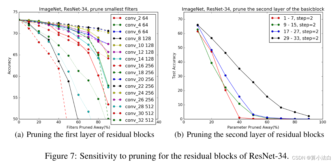
图 7：ResNet-34 残差块的剪枝敏感性。

4.4 COMPARISON WITH PRUNING RANDOM FILTERS AND LARGEST FILTERS

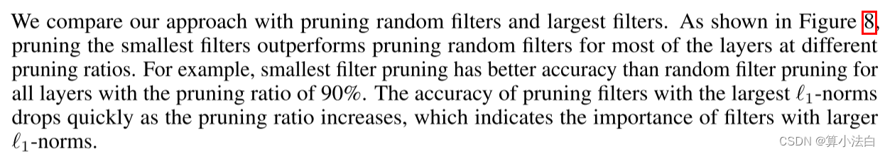
我们将我们的方法与修剪随机过滤器和最大过滤器进行比较。如图 8 所示，对于大多数层，在不同的剪枝比率下，剪枝最小过滤器的性能优于剪枝随机过滤器。例如，对于剪枝率为 90% 的所有层，最小滤波器剪枝比随机滤波器剪枝具有更好的精度。随着剪枝率的增加，具有最大1-范数的剪枝滤波器的准确度迅速下降，这表明具有较大1-范数的滤波器的重要性。

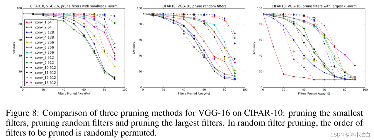
图 8：VGG-16 在 CIFAR-10 上的三种剪枝方法的比较：剪枝最小过滤器、剪枝随机过滤器和剪枝最大过滤器。在随机滤波器剪枝中，要剪枝的滤波器的顺序是随机排列的。

4.5 COMPARISON WITH ACTIVATION-BASED FEATURE MAP PRUNING

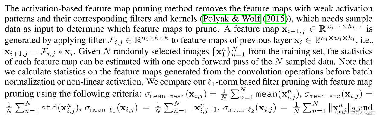
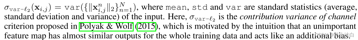
基于激活的特征图修剪方法去除了具有弱激活模式的特征图及其相应的过滤器和内核（Polyak＆Wolf（2015）），该方法需要样本数据作为输入来确定要修剪哪些特征图。通过将过滤器 Fi,j ∈ Rni×k×k 应用于前一层 xi ∈ Rni×wi×hi 的特征图（即 xi+1），生成特征图 xi+1,j ∈ Rwi+1×hi+1， j=Fi,j*xi。给定从训练集中随机选择的 N 张图像 {xn 1 }N n=1，每个特征图的统计信息可以通过 N 个采样数据的一个 epoch 前向传递来估计。请注意，我们在批量归一化或非线性激活之前计算由卷积操作生成的特征图的统计数据。我们使用以下标准将基于 1-范数的滤波器剪枝与特征图剪枝进行比较： σmean-mean(xi,j) = 1 N N n=1mean(xn i,j), σmean-std(xi,j) ) = 1 N N n=1 std(xn i,j), σmean-1(xi,j) = 1 N N n=1 xn i,j1, σmean-2(xi,j) ) = 1 N N n=1 xn i,j2 且 σvar-2(xi,j) = var({xn i,j2}N n=1)，其中mean、std 和var 是标准统计量（平均值、 输入的标准差和方差）。这里，σvar-2 是通道的贡献方差 Polyak & Wolf (2015) 中提出的标准，其动机是直觉认为不重要的 特征图对于整个训练数据具有几乎相似的输出，并且充当附加偏差。

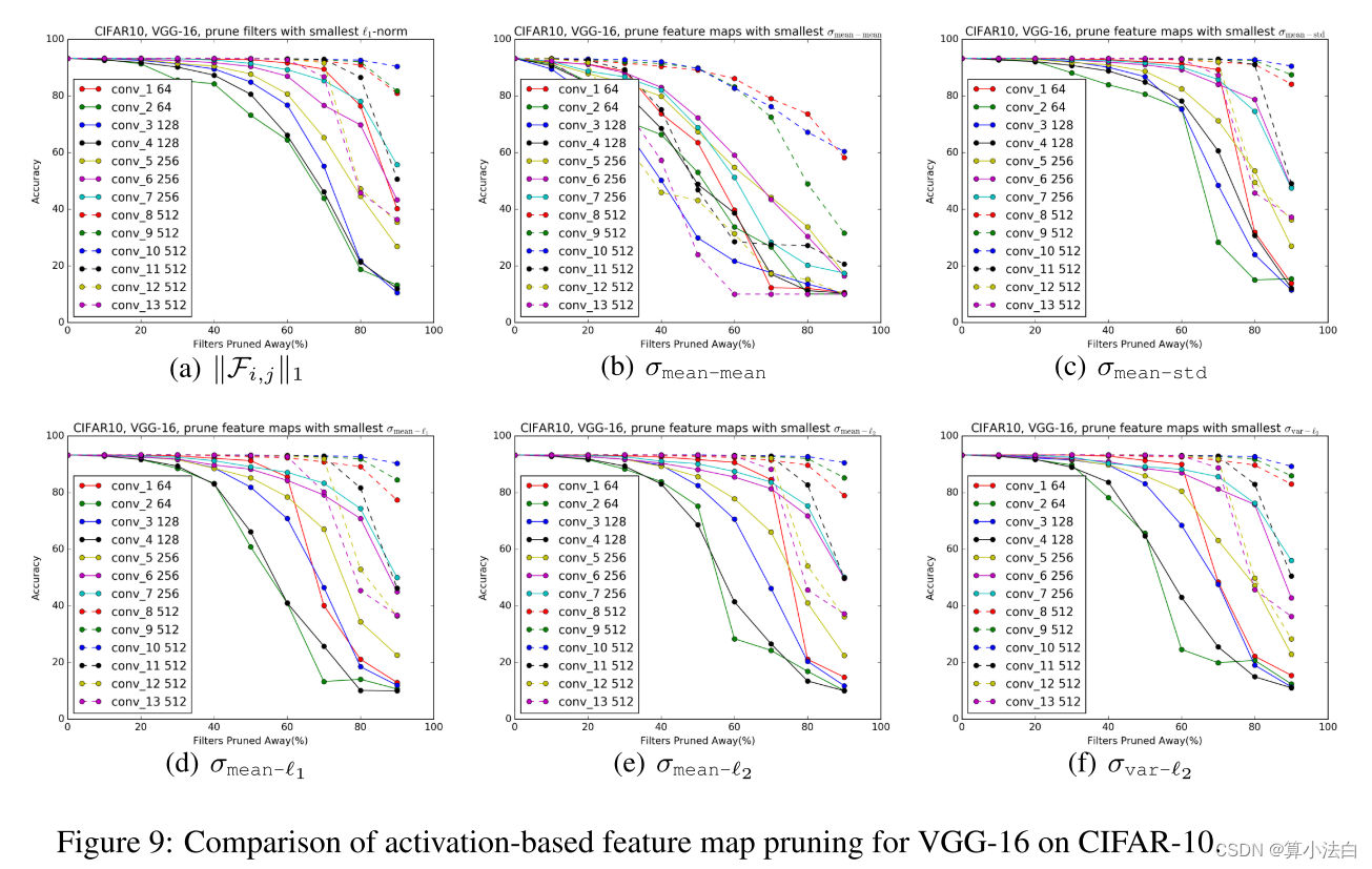
图 9：CIFAR-10 上 VGG-16 基于激活的特征图修剪的比较。

当使用更多样本数据时，标准的估计变得更加准确。在这里，我们使用整个训练集（CIFAR-10 的 N = 50, 000）来计算统计数据。使用上述标准对每层进行特征图剪枝的性能如图 9 所示。最小滤波器剪枝优于使用标准 σmean-mean、σmean-l1 、σmean-l2 和 σvar-l2 的特征图剪枝。 σmean-std 准则在剪枝率为 60% 的情况下具有与 l1-范数更好或相似的性能。然而，此后其性能迅速下降，特别是对于 conv 1、conv 2 和 conv 3 层。我们发现 l1-norm 考虑到它是无数据的，对于滤波器选择来说是一个很好的启发式。

5 CONCLUSIONS(结论)

Modern CNNs often have high capacity with large training and inference costs. In this paper we
present a method to prune filters with relatively low weight magnitudes to produce CNNs with
reduced computation costs without introducing irregular sparsity. It achieves about 30% reduction in FLOP for VGGNet (on CIFAR-10) and deep ResNets without significant loss in the original accuracy. Instead of pruning with specific layer-wise hayperparameters and time-consuming iterative retraining, we use the one-shot pruning and retraining strategy for simplicity and ease of implementation. By performing lesion studies on very deep CNNs, we identify layers that are robust or sensitive to pruning, which can be useful for further understanding and improving the architectures.

现代 CNN 通常具有较高的容量，但训练和推理成本较高。在本文中，我们提出了一种修剪权重相对较低的滤波器的方法，以生成具有降低计算成本的 CNN，且不会引入不规则稀疏性。它使 VGGNet（在 CIFAR-10 上）和深度 ResNet 的 FLOP 降低了约 30%，而原始精度没有显着损失。我们没有使用特定的逐层干草参数进行剪枝和耗时的迭代再训练，而是使用一次性剪枝和再训练策略，以实现简单性和易于实施。通过对非常深的 CNN 进行损伤研究，我们识别出稳健或对剪枝敏感的层，这对于进一步理解和改进架构很有用。

ACKNOWLEDGMENTS(致谢)

The authors would like to thank the anonymous reviewers for their valuable feedback.

作者要感谢匿名审稿人的宝贵反馈。