应用matlab的基础训练（1）—— 连续信号的波形频谱仿真

汗水会为王冠加冕

于 2023-03-13 22:57:26 发布

阅读量4.8k

点赞数 8

文章标签： matlab 开发语言

本文链接：https://blog.csdn.net/m0_68278088/article/details/129503573

版权

对于连续信号可分为周期信号和非周期信号，常见的连续非周期信号有双边指数函数、单边指数函数、矩形脉冲信号、钟形脉冲信号、符号函数、升余弦脉冲信号。常见的连续周期信号有正弦函数、余弦函数、方波、三角波。时域的周期性会使频谱是离散谱，而非周期性对应频域就是连续谱。下面我们可以明显看到两种类型信号谱的不同：

（1）连续非周期信号的时域表达式及幅度谱表达式

1.双边指数函数 f=exp(-1*abs(t)）、|F(w)|= $\frac{2}{1+w^{2}}$

2.单边指数函数 f=exp(-1*t).*heaviside(t)、|F(w)|= $\tfrac{}{}$ $\tfrac{1}{({1+w^{2}})^{1/2}}$

3.矩形脉冲信号 f=3*ones(size(t)).*and(t>=-2,t<=2)、|F(w)|=12|Sa(2w)|

4.钟形脉冲信号 f=5*exp(-(t/4).^2)、|F(w)|=20 $\sqrt{pi}$ * $\small e^{-4w^{2}}$

5.符号函数 f=1*heaviside(t)-1*heaviside(-t)、|F(w)|= $\small \frac{2}{|w|}$

6.升余弦脉冲信号 f=5/2*(1+cos(pi*t/4)).*((0<=abs(t))&(abs(t)<=4))、|F(w)|= $\small \frac{10sa(4w)}{1-(\frac{4w}{pi})^{2}}$

（2）连续周期信号的表达式和幅度谱特征

1.正弦函数 f=5/2*sin(pi*t*4); 周期为1/2，在正半轴频率为2的时候会有冲击。

2.余弦函数 f=5/2*cos(pi*t*4); 周期为1/2，在正半轴频率为2的时候会有冲击。

3.方波 f=square(pi*t); 周期为2，傅里叶级数为奇次谐波，且幅度会逐渐减小，所以在频率为0.5、1.5 、2.5等均有周期为1的离散谱。

4.三角波 f=sawtooth(0.5*pi*t,0.5); 周期为4，傅里叶级数同为奇次谐波，幅度以平方衰减，衰减更快，在频率为0.25、0.75 、1.25等均有周期为0.5的离散谱。

接下来让我们看看两种信号对应时域图和频谱图

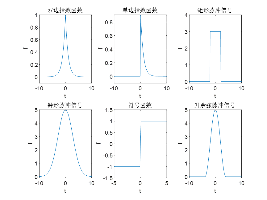
典型连续时间非周期信号时域波形

典型连续时间非周期信号频谱

连续时间周期信号时域波形

连续时间周期信号频谱

思考总结：matlab编写程序时，不需要申明变量，使用起来很方便，上手起来也比其它软件更快速。在画时域图和频谱图的时候最重要的是一些函数的使用，例如阶跃函数heaviside，方波函数square，三角波函数sawtooth。在画频谱会用到fourier和fft。连续时间非周期信号的频谱是一个连续谱，而周期信号的频谱是一个离散谱，如果信号在时域集中于有限的范围，在频域中会无限延伸。

fourier是算符号表达式的傅里叶变换，fft是算有限长离散序列的离散傅里叶变换的。对于连续时间非周期信号用fourier函数，应用fourier函数画频谱时应注意自变量t的数据类型，先开始我将t定义为t=-10:0.1:10，编辑器报错，后来将t改为syms t,系统默认为double类型，编译成功，我觉得发生错误的主要原因还是fourier函数的使用不当，它是对连续的时间信号进行傅里叶变换，所以时间是要连续，如果是t=-10:0.1:10，时间的取值是离散的。而且当时我写双边指数函数等后面几个函数时用的都是分段函数写法，进行傅里叶变换的时候，这种表达式编译器不会执行，结果也会出错，使用abs heaviside 这些后才能编译成功。例如f=exp(1*t).*(t<0)+exp(-1*t).*(t>=0); 和改正后f=exp(-1*abs(t));

在对连续时间周期信号进行傅里叶变换时用fft,所以要确定采样间隔和频谱，根据奈奎斯特定理，采样频率大于信号频率的两倍。但对与fft的原理不是很了解，方波，三角波的主峰所在的频率点符合理论值，正余弦信号的冲击点处也符合理论值。

附代码如下：

%典型连续时间非周期信号时域波形

clc;

clear;

close all;

subplot(2,3,1);

t=-10:0.1:10;

f=exp(-1*abs(t));

plot(t,f);

xlabel('t');

ylabel('f');

title("双边指数函数");

subplot(2,3,2);

t=-10:0.1:10;

f=exp(-1*t).*heaviside(t);

plot(t,f);

xlabel('t');

ylabel('f');

title("单边指数函数");

subplot(2,3,3);

t=-10:0.1:10;

f=3*ones(size(t)).*and(t>=-2,t<=2);

plot(t,f);

xlabel('t');

ylabel('f');

title("矩形脉冲信号");

subplot(2,3,4);

t=-10:0.1:10;

f=5*exp(-(t/4).^2);

plot(t,f);

xlabel('t');

ylabel('f');

title("钟形脉冲信号");

axis([-10 10 0 4]);

subplot(2,3,5);

t=-10:0.1:10;

f=1*heaviside(t)-1*heaviside(-t);

plot(t,f);

xlabel('t');

ylabel('f');

axis([-5 5 -1.5 1.5]);

title("符号函数");

subplot(2,3,6);

t=-10:0.1:10;

f=5/2*(1+cos(pi*t/4)).*((0<=abs(t))&(abs(t)<=4));

plot(t,f);

xlabel('t');

ylabel('f');

title("升余弦脉冲信号");

%典型连续时间非周期信号频谱

clc;

clear;

close all;

syms t;

subplot(2,3,1);

f=exp(-1*abs(t));

F=fourier(f);

ezplot(F);

xlabel('w');

ylabel('F');

title("双边指数函数");

subplot(2,3,2);

f=exp(-1*t).*heaviside(t);

F=fourier(f);

ezplot(abs(F));

xlabel('w');

ylabel('F');

title("单边指数函数");

subplot(2,3,3);

f=3*(heaviside(t+2)-heaviside(t-2));

F=fourier(f);

ezplot(abs(F));

xlabel('w');

ylabel('F');

title("矩形脉冲信号");

subplot(2,3,4);

f=5*exp(-(t/4).^2);

F=fourier(f);

ezplot(abs(F));

xlabel('w');

ylabel('F');

title("钟形脉冲信号");

subplot(2,3,5);

f=1*heaviside(t)-1*heaviside(-t);

F=fourier(f);

ezplot(abs(F));

xlabel('w');

ylabel('F');

axis([-5 5 0 50]);

title("符号函数");

subplot(2,3,6);

f=5/2*(1+cos(pi*t/4)).*(heaviside(t+4)-heaviside(t-4));

F=fourier(f);

ezplot(abs(F));

xlabel('w');

ylabel('F');

axis([-5 5 0 22]);

title("升余弦脉冲信号");

%连续时间周期信号时域波形

clc;

clear;

close all;

subplot(2,2,1);

t=-10:0.1:10;

f=5/2*sin(pi*t*4);

plot(t,f);

xlabel('t');

ylabel('f');

title("正弦函数");

subplot(2,2,2);

t=-10:0.1:10;

f=5/2*cos(pi*t*4);

plot(t,f);

xlabel('t');

ylabel('f');

title("余弦函数");

subplot(2,2,3);

t=-10:0.01:10;

f=square(pi*t);

plot(t,f);

xlabel('t');

ylabel('f');

title("方波");

subplot(2,2,4);

t=-10:0.01:10;

axis([-2 2 -2 2]);

f=sawtooth(0.5*pi*t,0.5);

plot(t,f);

xlabel('t');

ylabel('f');

title("三角波");

%连续时间周期信号频谱

clc;

clear;

close all;

subplot(2,2,1);

t=-10:0.01:10;

f=5/2*sin(pi*t/4);

fs=100;

L = length(t);

n = 2^nextpow2(L);

Y = abs(fft(f,n));

f = fs*(0:(n/2))/n;

plot(f,Y(1:n/2+1)) ;

xlabel('w');

ylabel('F');

axis([-5 60 0 2000]);

title("正弦波");

subplot(2,2,2);

t=-10:0.01:10;

f=5/2*cos(pi*t/4);

fs=100;

L = length(t);

n = 2^nextpow2(L);

Y = abs(fft(f,n));

f = fs*(0:(n/2))/n;

plot(f,Y(1:n/2+1)) ;

xlabel('w');

ylabel('F');

axis([-5 60 0 2000]);

title("余弦波");

subplot(2,2,3);

t=-10:0.1:10;

f=square(pi*t);

fs=10;

L = length(t);

n = 2^nextpow2(L);

Y = abs(fft(f,n));

f = fs*(0:(n/2))/n;

plot(f,Y(1:n/2+1)) ;

xlabel('w');

ylabel('F');

title("方波");

subplot(2,2,4);

t=-10:0.1:10;

f=sawtooth(0.5*pi*t,0.5);

fs=10;

L = length(t);

n = 2^nextpow2(L);

Y = abs(fft(f,n));

f = fs*(0:(n/2))/n;

plot(f,Y(1:n/2+1)) ;

xlabel('w');

ylabel('F');

title("三角波");

汗水会为王冠加冕

关注

8
点赞
踩
45

收藏

觉得还不错? 一键收藏
0
评论
应用matlab的基础训练（1）—— 连续信号的波形频谱仿真

编辑器报错，后来将t改为syms t,系统默认为double类型，编译成功，我觉得发生错误的主要原因还是fourier函数的使用不当，它是对连续的时间信号进行傅里叶变换，所以时间是要连续，如果是t=-10:0.1:10，时间的取值是离散的。6.升余弦脉冲信号 f=5/2*(1+cos(pi*t/4)).*((0<=abs(t))&(abs(t)<=4))、|F(w)|=3.矩形脉冲信号 f=3*ones(size(t)).*and(t>=-2,t<=2)、|F(w)|=12|Sa(2w)|
复制链接

扫一扫