Python Matplotlib 指南

目录

1. 为什么要学Matplotlib？
2. 快速安装与验证
3. 你的第一个图表
4. 核心概念解析
5. 基础图表大全
   • 5.1 八大基础图表
   • 5.2 十大进阶图表详解
   • 5.3 组合图表技巧
6. 图表定制技巧
   • 6.1 样式参数全解
   • 6.2 颜色与样式进阶
7. 多图布局系统
   • 7.1 基础子图布局
   • 7.2 高级布局技巧
   • 7.3 嵌套子图系统
8. 3D与高级图表
   • 8.1 3D柱状图
   • 8.2 3D曲面动画
9. 动态可视化
   • 9.1 实时数据流
   • 9.2 保存动画文件
10. 实战案例
    • 10.1 股票数据分析
    • 10.2 实时数据仪表盘
    • 10.3 地理信息可视化
    • 10.4 机器学习可视化
11. 常见问题排雷
    • 11.1 图表显示问题
    • 11.2 中文显示设置
    • 11.3 高级问题解决
12. 样式美化终极指南
    • 12.1 预置样式速查
    • 12.2 制作主题模板
13. 高效工作流建议
    • 13.1 调试可视化
    • 13.2 版本控制技巧

---

1. 为什么要学Matplotlib？

1.1 数据可视化的重要性

• 人类视觉处理速度比文本快6万倍
• 70%的大脑神经元参与视觉处理
• 数据科学家的日常工作50%与可视化相关

1.2 Matplotlib的优势

import matplotlib.pyplot as plt
import numpy as np

# 三行代码快速绘图
x = np.linspace(0, 2*np.pi, 100)
plt.plot(x, np.sin(x))
plt.show()

支持30+种图表类型、高度可定制、完美集成NumPy

---

2. 快速安装与验证

2.1 安装方法

# 基础安装
pip install matplotlib

# 完整安装（包含所有依赖）
pip install "matplotlib[all]"

2.2 环境验证

import matplotlib
print(matplotlib.__version__)  # 应显示3.5.0以上版本
print(matplotlib.get_backend()) # 查看当前后端

---

3. 你的第一个图表

3.1 折线图完整流程

# 准备数据
x = [1, 2, 3, 4, 5]
y = [2, 4, 6, 8, 10]

# 创建画布
plt.figure(figsize=(8,4), dpi=100)

# 绘制图形
plt.plot(x, y, 
         color='red', 
         linestyle='--', 
         marker='o', 
         label='Linear')

# 添加装饰
plt.title("第一个折线图示例", fontsize=14)
plt.xlabel("X轴", fontsize=12)
plt.ylabel("Y轴", fontsize=12)
plt.grid(alpha=0.5)
plt.legend()

# 显示/保存
plt.savefig('first_plot.png', bbox_inches='tight')
plt.show()

3.2 新手常见错误

• 忘记plt.show()导致不显示图表
• 中文显示乱码问题
• 图形元素遮挡问题
• 混淆figure和axes对象

---

4. 核心概念解析

4.1 对象层次结构

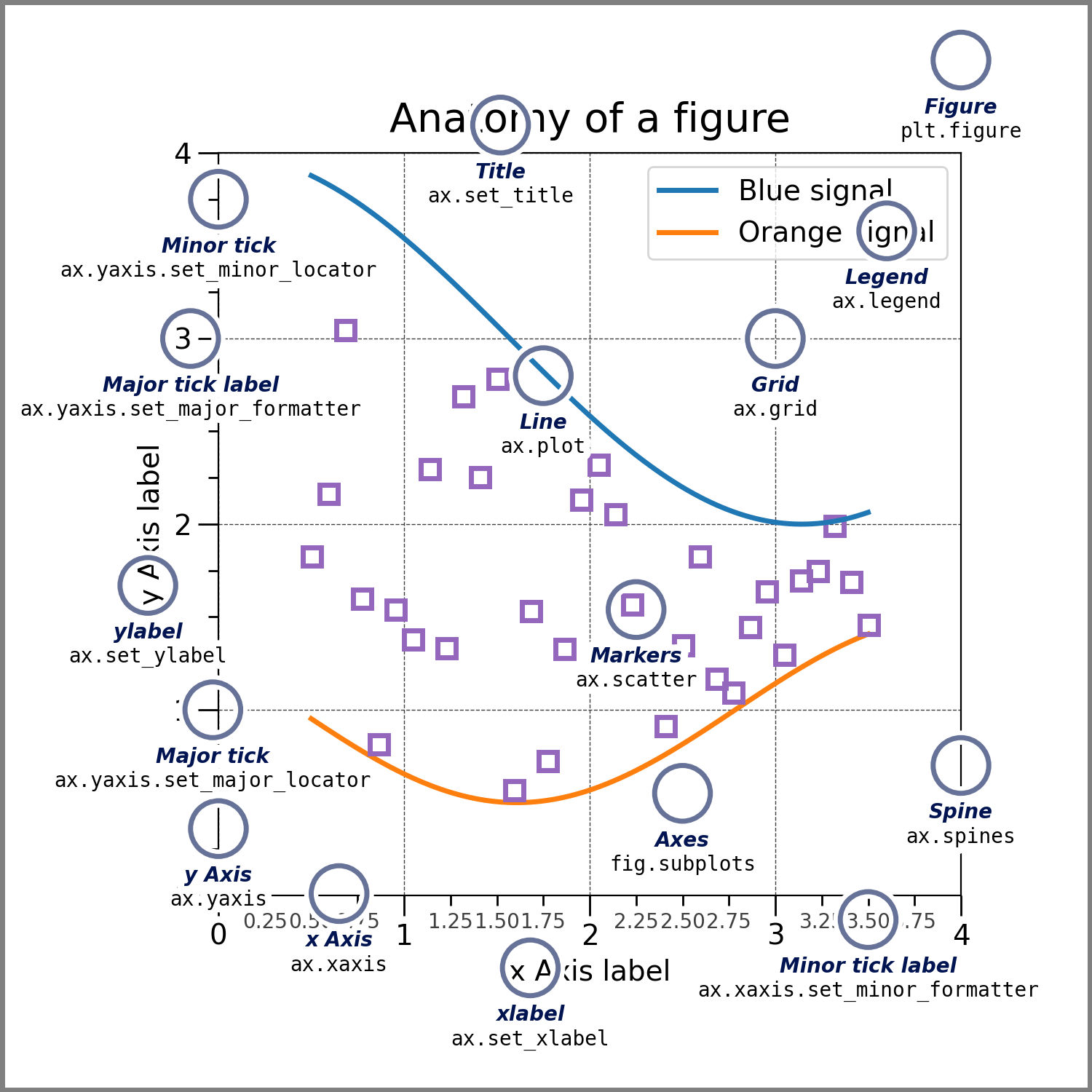
• Figure：顶级容器（相当于画布）
• Axes：坐标系（真正绘制图表的区域）
• Axis：坐标轴
• Artist：所有可见元素（线条、文本等）

4.2 两种编程风格

pyplot风格（快速绘图）

plt.plot([1,2,3], [4,5,6])
plt.title("快速绘图")
plt.show()

面向对象风格（推荐）

fig, ax = plt.subplots()
ax.plot([1,2,3], [4,5,6])
ax.set_title("面向对象方式")
fig.show()

---

5. 基础图表大全

5.1 八大基础图表

# 数据准备
x = np.linspace(0, 10, 100)
y = np.sin(x)

# 创建2x4子图
fig, axs = plt.subplots(2,4, figsize=(16,8))

# 折线图
axs[0,0].plot(x, y)
axs[0,0].set_title('Line plot')

# 散点图
axs[0,1].scatter(x, y, c='red', s=10)
axs[0,1].set_title('Scatter plot')

# 柱状图
axs[0,2].bar(['A','B','C'], [3,7,2])
axs[0,2].set_title('Bar chart')

# 直方图
axs[0,3].hist(np.random.randn(1000), bins=30)
axs[0,3].set_title('Histogram')

# 饼图
axs[1,0].pie([30,40,30], labels=['A','B','C'])
axs[1,0].set_title('Pie chart')

# 箱线图
axs[1,1].boxplot([np.random.normal(0,1,100)])
axs[1,1].set_title('Box plot')

# 热力图
im = axs[1,2].imshow(np.random.rand(10,10))
plt.colorbar(im, ax=axs[1,2])
axs[1,2].set_title('Heatmap')

# 面积图
axs[1,3].fill_between(x, y, alpha=0.5)
axs[1,3].set_title('Area chart')

plt.tight_layout()
plt.show()

5.2 十大进阶图表详解

5.2.1 堆叠柱状图

labels = ['第一季度', '第二季度', '第三季度', '第四季度']
sales_A = [23, 45, 15, 32]
sales_B = [34, 30, 26, 40]

fig, ax = plt.subplots()
ax.bar(labels, sales_A, label='产品A')
ax.bar(labels, sales_B, bottom=sales_A, label='产品B')

ax.set_title('季度销售额对比')
ax.legend()
plt.show()

应用场景：比较多个分类的组成结构
关键参数：bottom设置堆叠基准，hatch添加纹理样式

5.2.2 水平条形图

categories = ['苹果', '香蕉', '橙子', '葡萄']
values = [85, 67, 92, 45]

fig, ax = plt.subplots()
ax.barh(categories, values, color='skyblue')
ax.set_xlabel('销量（万斤）')
ax.set_title('水果销量排行榜')

适用情况：类别名称较长时，或需要直观排名时
调整技巧：使用invert_yaxis()反转顺序

5.2.3 误差棒图

x = np.arange(5)
y = [12, 15, 14, 13, 16]
error = [1.5, 2.1, 0.9, 1.2, 1.8]

fig, ax = plt.subplots()
ax.errorbar(x, y, yerr=error, fmt='o', 
           capsize=5, ecolor='red')
ax.set_xticks(x)
ax.set_xticklabels(['实验1', '实验2', '实验3', '实验4', '实验5'])

核心参数：

• yerr/xerr: 误差范围
• fmt: 数据点样式（'o’表示圆圈）
• capsize: 误差棒端帽大小

5.2.4 极坐标图

theta = np.linspace(0, 2*np.pi, 8)
r = np.random.randint(1, 10, 8)

fig = plt.figure()
ax = fig.add_subplot(111, projection='polar')
ax.plot(theta, r, marker='*', color='purple')
ax.fill(theta, r, alpha=0.3)
ax.set_title('雷达图示例', pad=20)

适用领域：方向数据、周期性数据可视化
注意事项：角度单位为弧度制

5.2.5 分簇散点图

np.random.seed(42)
data1 = np.random.normal(0, 1, 50)
data2 = np.random.normal(3, 1.5, 50)

fig, ax = plt.subplots()
ax.scatter(np.ones(50), data1, label='组A')
ax.scatter(np.ones(50)*2, data2, label='组B')

ax.set_xticks([1,2])
ax.set_xticklabels(['对照组', '实验组'])
ax.legend()

可视化效果：清晰展示组间数据分布差异
增强技巧：添加抖动jitter防止点重叠

5.2.6 六边形箱图

x = np.random.normal(0, 1, 1000)
y = x * 2 + np.random.normal(0, 1, 1000)

fig, ax = plt.subplots()
hb = ax.hexbin(x, y, gridsize=30, cmap='Blues')
fig.colorbar(hb)
ax.set_title('二维数据密度分布')

适用场景：大数据集的密度可视化
关键参数：gridsize控制六边形数量，bins设置颜色分级

5.2.7 等高线图

x = np.linspace(-3, 3, 100)
y = np.linspace(-3, 3, 100)
X, Y = np.meshgrid(x, y)
Z = np.sin(X**2 + Y**2)

fig, ax = plt.subplots()
contour = ax.contour(X, Y, Z, levels=10, cmap='RdYlBu')
ax.clabel(contour, inline=True)
ax.set_title('二维函数等高线')

应用领域：地理信息、数学函数可视化
扩展技巧：使用contourf创建填充等高线

5.2.8 矢量场图

x, y = np.meshgrid(np.arange(0, 2*np.pi, 0.5),
                   np.arange(0, 2*np.pi, 0.5))
U = np.cos(x)
V = np.sin(y)

fig, ax = plt.subplots()
ax.quiver(x, y, U, V, scale=20, color='green')
ax.set_title('矢量场示意图')

适用场景：流体力学、电磁场可视化
参数解析：scale控制箭头大小，units设置单位类型

5.3 组合图表技巧

fig, ax = plt.subplots()

# 主坐标系绘制折线图
x = np.linspace(0, 10, 100)
ax.plot(x, np.sin(x), color='blue', label='正弦波')

# 创建副坐标系
ax2 = ax.twinx()
ax2.plot(x, np.exp(-x), color='red', label='指数衰减')

# 统一图例
lines = ax.get_lines() + ax2.get_lines()
ax.legend(lines, [l.get_label() for l in lines])

ax.set_title('双坐标系组合图')
plt.show()

组合要点：

1. 使用twinx()创建共享x轴的第二个坐标系
2. 统一坐标范围避免比例失调
3. 合并不同坐标系的图例

---

6. 图表定制技巧

6.1 样式参数全解

# 通用参数设置模板
plt.style.use('seaborn')  # 使用预定义样式

fig, ax = plt.subplots(figsize=(10,6))

ax.plot(x, y,
        linewidth=2,      # 线宽
        linestyle='-.',    # 线型（实线、虚线等）
        marker='s',       # 标记形状
        markersize=8,     # 标记尺寸
        markerfacecolor='white',  # 标记填充色
        markeredgecolor='red',    # 标记边框色
        markeredgewidth=1.5,      # 边框宽度
        alpha=0.8)        # 透明度

ax.set_title('定制化图表示例', 
            fontsize=16, 
            fontweight='bold',
            color='navy')

ax.set_xlabel('时间轴', 
             fontsize=12,
             labelpad=10)  # 标签与坐标轴的间距

ax.tick_params(axis='both',  # 坐标轴刻度设置
              which='major',
              direction='out',
              length=6,
              width=1.5,
              colors='gray',
              labelsize=10)

ax.grid(True, 
       linestyle=':',
       linewidth=0.8,
       alpha=0.7)

6.2 颜色与样式进阶

# 颜色选择方法
ax.plot(x, y, 
       color='#2ca02c',      # HEX格式
       color=(0.1,0.5,0.8),  # RGB元组（0-1范围）
       color='chartreuse')    # 英文颜色名称

# 使用colormap
gradient = np.linspace(0, 1, 100)
ax.scatter(x, y, c=gradient, cmap='viridis')

# 自定义线型
ax.plot(x, y, 
       linestyle=(0, (3, 1, 1, 1)),  # 自定义虚线模式
       dash_capstyle='round')         # 虚线端点样式

---

7. 多图布局系统

7.1 基础子图布局

# 创建2行3列的子图网格
fig, axs = plt.subplots(nrows=2, ncols=3, figsize=(12,8))

# 在指定位置绘制图表
axs[0,0].plot(x, np.sin(x))
axs[1,2].scatter(x, np.cos(x))

# 共享坐标轴
fig, (ax1, ax2) = plt.subplots(2, 1, sharex=True)

7.2 高级布局技巧

import matplotlib.gridspec as gridspec

# 创建复杂布局
fig = plt.figure(constrained_layout=True)
gs = gridspec.GridSpec(3, 3, figure=fig)

# 跨行/列布局
ax1 = fig.add_subplot(gs[0, :])  # 首行全宽
ax2 = fig.add_subplot(gs[1:, 0]) # 右侧两行第一列
ax3 = fig.add_subplot(gs[1:, 1:]) # 右下区域

# 添加间距控制
plt.subplots_adjust(wspace=0.4, hspace=0.3)

7.3 嵌套子图系统

# 主图内部插入子图
fig, ax = plt.subplots()
inset_ax = ax.inset_axes([0.6, 0.6, 0.3, 0.3])  # [x, y, width, height]

# 主图绘制散点图
ax.scatter(x, y)

# 子图显示局部放大
inset_ax.plot(x_detail, y_detail)

---

8. 3D与高级图表

8.1 3D柱状图

fig = plt.figure()
ax = fig.add_subplot(111, projection='3d')

xpos = [1,2,3,4,5]
ypos = [1,2,3,4,5]
zpos = np.zeros(5)

dx = dy = 0.5  # 柱体底面尺寸
dz = [1,2,3,4,5]  # 高度值

ax.bar3d(xpos, ypos, zpos, dx, dy, dz, 
        color='#00ceaa', 
        edgecolor='black')

ax.set_xlabel('X轴')
ax.set_ylabel('Y轴')
ax.set_zlabel('Z轴')

8.2 3D曲面动画

from matplotlib.animation import FuncAnimation

fig = plt.figure()
ax = fig.add_subplot(111, projection='3d')

X = np.arange(-5, 5, 0.25)
Y = np.arange(-5, 5, 0.25)
X, Y = np.meshgrid(X, Y)

def init():
    Z = np.sin(np.sqrt(X**2 + Y**2))
    surf = ax.plot_surface(X, Y, Z, cmap='viridis')
    return fig,

def animate(i):
    ax.cla()
    Z = np.sin(np.sqrt(X**2 + Y**2) + 0.1*i)
    surf = ax.plot_surface(X, Y, Z, cmap='viridis')
    return fig,

ani = FuncAnimation(fig, animate, init_func=init, frames=50)
plt.show()

---

9. 动态可视化

9.1 实时数据流

import random
from itertools import count

plt.ion()  # 开启交互模式
fig, ax = plt.subplots()

x = []
y = []
index = count()

def update():
    x.append(next(index))
    y.append(random.randint(0, 10))
    ax.cla()
    ax.plot(x, y, 'g-')
    ax.set_ylim(0,10)
    plt.pause(0.1)

for _ in range(50):
    update()

plt.ioff()
plt.show()

9.2 保存动画文件

# 生成动画对象
ani = FuncAnimation(fig, animate, frames=100)

# 保存为GIF（需要imagemagick）
ani.save('animation.gif', writer='imagemagick', fps=30)

# 保存为MP4（需要ffmpeg）
ani.save('animation.mp4', writer='ffmpeg', 
        fps=24, 
        dpi=200,
        bitrate=1800)

---

10. 实战案例（扩展篇）

10.1 股票数据分析

# 绘制K线图
from mplfinance.original_flavor import candlestick_ohlc

# 准备数据
data = [...] # 包含日期、开盘、最高、最低、收盘价

fig, ax = plt.subplots(figsize=(12,6))
candlestick_ohlc(ax, data, width=0.6)
ax.xaxis_date() # 转换日期格式
plt.title('股票K线图')
plt.xlabel('日期')
plt.ylabel('价格')

10.2 实时数据仪表盘

import time

plt.ion() # 启用交互模式
fig, ax = plt.subplots()

for i in range(50):
    y = np.random.rand()
    ax.scatter(i, y, c='blue')
    ax.set_xlim(0,50)
    plt.pause(0.1) # 暂停0.1秒

plt.ioff()
plt.show()

10.3 地理信息可视化

import cartopy.crs as ccrs

fig = plt.figure(figsize=(10,6))
ax = fig.add_subplot(1, 1, 1, projection=ccrs.PlateCarree())

ax.coastlines()
ax.gridlines()
ax.add_feature(cartopy.feature.LAND)
ax.add_feature(cartopy.feature.OCEAN)

# 绘制城市位置
cities = {
    '北京': (116.4, 39.9),
    '上海': (121.4, 31.2),
    '广州': (113.3, 23.1)
}

for city, (lon, lat) in cities.items():
    ax.plot(lon, lat, 'ro', markersize=8, transform=ccrs.Geodetic())
    ax.text(lon+2, lat, city, transform=ccrs.Geodetic())

10.4 机器学习可视化

from sklearn.datasets import make_moons
from sklearn.cluster import KMeans

# 生成数据
X, y = make_moons(200, noise=0.1)

# 聚类分析
kmeans = KMeans(n_clusters=2)
labels = kmeans.fit_predict(X)

# 可视化结果
fig, ax = plt.subplots()
scatter = ax.scatter(X[:,0], X[:,1], c=labels, cmap='Set2', s=50)

# 绘制决策边界
h = 0.02
x_min, x_max = X[:,0].min()-1, X[:,0].max()+1
y_min, y_max = X[:,1].min()-1, X[:,1].max()+1
xx, yy = np.meshgrid(np.arange(x_min, x_max, h),
                    np.arange(y_min, y_max, h))
Z = kmeans.predict(np.c_[xx.ravel(), yy.ravel()])
Z = Z.reshape(xx.shape)

ax.contourf(xx, yy, Z, alpha=0.2, cmap='Set2')
ax.set_title('K均值聚类可视化')

---

11. 常见问题排雷（扩展篇）

Q：为什么图表显示空白？
A：检查是否缺少plt.show()，或在使用Jupyter时忘记%matplotlib inline

Q：如何显示中文标签？

plt.rcParams['font.sans-serif'] = ['SimHei'] # Windows
plt.rcParams['font.sans-serif'] = ['Arial Unicode MS'] # Mac
plt.rcParams['axes.unicode_minus'] = False # 解决负号显示

Q：如何保存高清大图？

plt.savefig('output.png', 
           dpi=300, 
           bbox_inches='tight', 
           facecolor='white')

Q：如何调整图例位置和样式？

ax.legend(loc='upper right',         # 10个预设位置
         bbox_to_anchor=(1.3, 0.5), # 自定义位置
         frameon=False,             # 移除边框
         ncol=2,                    # 分列显示
         title='图例标题',
         title_fontsize='large')

Q：如何处理大数据集显示卡顿？

# 优化策略：
# 1. 使用rasterized=True参数矢量化部分元素
ax.plot(x, y, rasterized=True)

# 2. 降低采样率
downsample = slice(None, None, 10)
ax.plot(x[downsample], y[downsample])

# 3. 使用快速渲染后端
import matplotlib
matplotlib.use('Agg')  # 非交互式后端

Q：如何创建自定义标记形状？

# 使用Unicode符号
ax.plot(x, y, marker='$\u2665$', markersize=15)

# 自定义路径
verts = [
    (0., -0.5),
    (0.5, 0.),
    (0., 0.5),
    (-0.5, 0.),
    (0., -0.5)
]
path = matplotlib.path.Path(verts)
ax.scatter(x, y, marker=path, s=500)

---

12. 样式美化终极指南

12.1 预置样式速查

# 查看所有可用样式
print(plt.style.available)
# ['classic', 'ggplot', 'seaborn', 'dark_background'...]

# 组合多个样式
plt.style.use(['seaborn-darkgrid', 'fast'])

# 自定义样式文件
plt.style.use('./custom.mplstyle')

12.2 制作主题模板

# 创建.mplstyle文件内容
'''
axes.facecolor: F0F0F0
figure.facecolor: FFFFFF
axes.grid: True
grid.color: DDDDDD
font.family: sans-serif
'''

# 应用自定义主题
plt.style.use('my_theme.mplstyle')

---

13. 高效工作流建议

13.1 调试可视化

# 快速查看对象属性
print(ax.properties())

# 交互式调试模式
plt.ion()  # 开启交互模式
fig.canvas.draw()  # 强制实时刷新

13.2 版本控制技巧

# 保存可复现的参数配置
with open('plot_config.json', 'w') as f:
    json.dump(plt.rcParams, f)

# 加载配置
with open('plot_config.json') as f:
    plt.rcParams.update(json.load(f))

---

终极提示：

1. 掌握快捷键提升效率（如s=保存，q=退出窗口）
2. 使用IPython魔法命令：%matplotlib auto/widget
3. 定期查看官方示例库：https://matplotlib.org/stable/gallery
4. 学习使用mplcursors实现数据光标提示
5. 探索第三方扩展库：mplot3d, seaborn, plotly

学习建议：每个示例至少手动输入一遍，尝试修改参数观察变化！