机器学习实验三

《机器学习与数据挖掘》实验三

实验题目：   求解对数几率回归问题                                             

实验目的：   掌握对数几率回归的基本原理与实现                                          

实验环境（硬件和软件）   Anaconda/Jupyter notebook/Pycharm                               

实验内容：

根据给定数据集（存放在data1.txt文件中，二分类数据），编码实现基于梯度下降的Logistic回归算法，并画出决策边界；

一、已经给定部分代码，补充完整的代码，需要补充代码的地方已经用红色字体标注，包括：

（1）#补充计算代价的代码；

（2）#补充参数更新代码；

（3）#补充画决策边界的代码；

二、提交的实验内容：（1）补充完整的代码；（也可以自己重写这部分的代码提交）（2）数据散点图，以及得到的决策边界；（3）梯度下降过程中损失的变化图；（4）基于训练得到的参数，输入新的样本数据，输出预测值；

import numpy as np

import matplotlib.pyplot as plt

import matplotlib as mpl

from sklearn.metrics import accuracy_score

def loaddata():

    data = np.loadtxt('data/data1.txt',delimiter=',')

    n = data.shape[1] - 1  # 特征数

    X = data[:, 0:n]

    y = data[:, -1].reshape(-1, 1)

return X, y

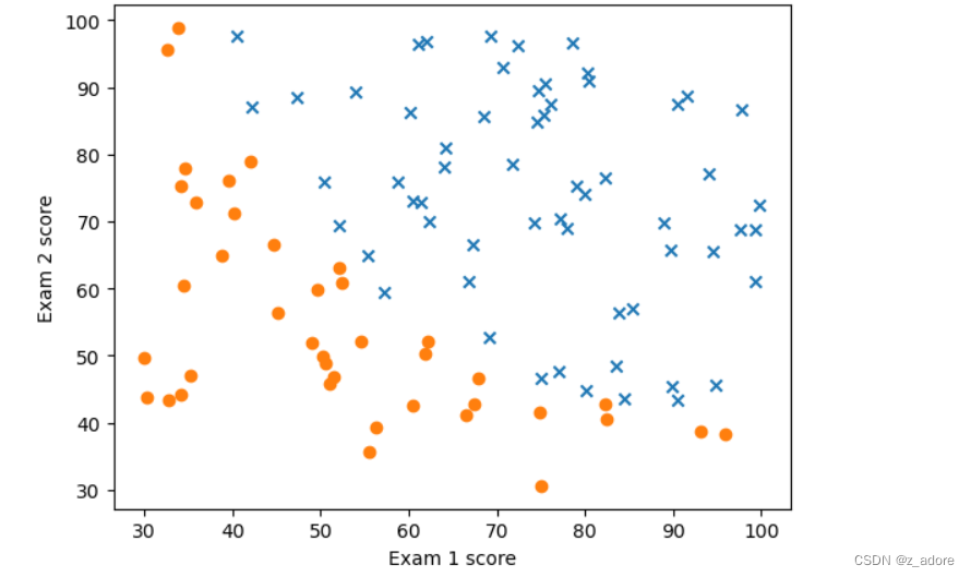
def plot(X,y):

    pos = np.where(y==1)

    neg = np.where(y==0)

    plt.scatter(X[pos[0],0],X[pos[0],1],marker='x')

    plt.scatter(X[neg[0], 0], X[neg[0], 1], marker='o')

    plt.xlabel('Exam 1 score')

    plt.ylabel('Exam 2 score')

plt.show()

X,y = loaddata()

plot(X,y)

print（X,y）

def sigmoid(z):

    r = 1/(1+np.exp(-z))

return r

def hypothesis(X,theta):

    z=np.dot(X,theta)

return sigmoid(z)

def computeCost(X,y,theta):

m = X.shape[0]

#补充计算代价的代码；

z=-1*y*np.log(hypothesis(X,theta))-(1-y)*np.log(1-hypothesis(X,theta))

return np.sum(z)/m

def gradientDescent(X,y,theta,iterations,alpha):

    #取数据条数

    m = X.shape[0]

    #在x最前面插入全1的列

    X = np.hstack((np.ones((m, 1)), X))

    for i in range(iterations):

#补充参数更新代码；

for j in range(len(theta)):

theta[j]=theta[j]-(alpha/m)*np.sum((hypothesis(X,theta)-y)*X[:,j].reshape(-1,1))

        theta = theta_temp

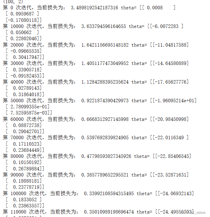
        #每迭代1000次输出一次损失值

        if(i%10000==0):

            print('第',i,'次迭代，当前损失为：',computeCost(X,y,theta),'theta=',theta)

return theta

def predict(X):

    # 在x最前面插入全1的列

    c = np.ones(X.shape[0]).transpose()

    X = np.insert(X, 0, values=c, axis=1) 

    #求解假设函数的值

    h = hypothesis(X,theta)

    #根据概率值决定最终的分类,>=0.5为1类，<0.5为0类

    h[h>=0.5]=1

    h[h<0.5]=0

return h

X,y = loaddata()

n = X.shape[1]#特征数

theta = np.zeros(n+1).reshape(n+1, 1)

# theta是列向量,+1是因为求梯度时X前会增加一个全1列

theta_temp = np.zeros(n+1).reshape(n+1, 1)

iterations = 250000

alpha = 0.008

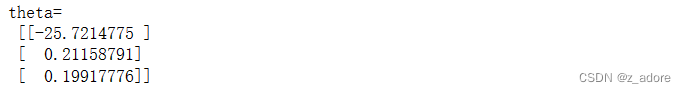
theta = gradientDescent(X,y,theta,iterations,alpha)

print('theta=\n',theta)

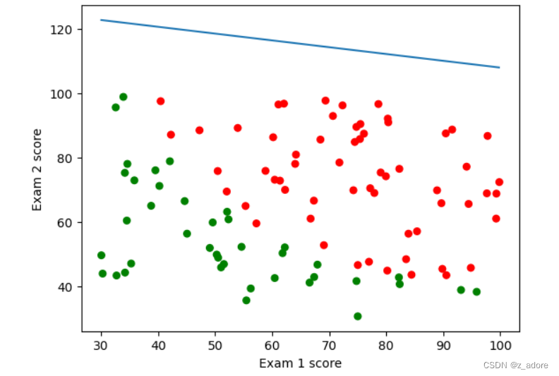
def plotDescisionBoundary(X,y,theta):

    cm_dark = mpl.colors.ListedColormap(['g', 'r'])

    plt.xlabel('Exam 1 score')

    plt.ylabel('Exam 2 score')

plt.scatter(X[:,0],X[:,1],c=np.array(y).squeeze(),cmap=cm_dark,s=30)

#补充画决策边界代码；

x1 = np.arange(min(X[:,0]),max(X[:,0]),0.1)

x2 = -(theta[1]*x1+theta[0]/theta[2])

    plt.plot(x1,x2)

plt.show()

plotDescisionBoundary(X,y,theta)

实验结果：

代码内容补充见上图红色标记处；

实验结果见如下：

部分数据显示：