利用RRCF包进行异常值检测

首先准备数据：

import rrcf
df.head(10)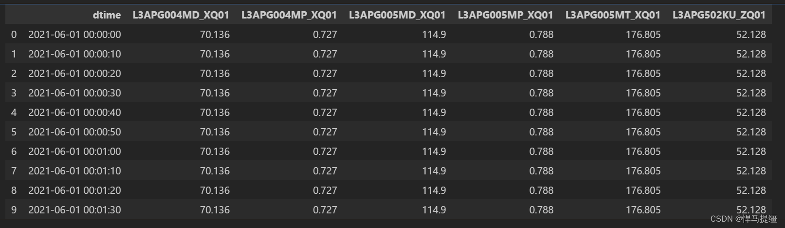

准备数据，去掉时间列

# 准备数据，去掉时间列
X = df.drop(columns=['dtime']).values

num_trees = 100
tree_size = 256
forest = []

# 存储每个点的索引以便之后计算CoDisp
indices = {}

for _ in range(num_trees):
    ixs = np.random.choice(len(X), size=tree_size, replace=False)
    tree = rrcf.RCTree()
    for ix in ixs:
        index = (ix, _)
        tree.insert_point(X[ix], index=index)
        if index not in indices:
            indices[index] = []
        indices[index].append(tree)
    forest.append(tree)

# 计算一致偏离度（CoDisp）
scores = np.zeros(len(X))

for ix in range(len(X)):
    total_codisp = 0
    for tree in forest:
        if (ix, _) in tree.leaves:
            codisp = tree.codisp((ix, _))
            total_codisp += codisp
    scores[ix] = total_codisp / num_trees

# 将分数添加到原始数据中
df['anomaly_score'] = scores

结果可视：

import matplotlib.pyplot as plt

plt.figure(figsize=(10, 6))
plt.plot(df['dtime'], df['anomaly_score'], label='Anomaly Score')
plt.xlabel('Time')
plt.ylabel('Anomaly Score')
plt.title('Anomaly Scores Over Time')
plt.legend()
plt.show()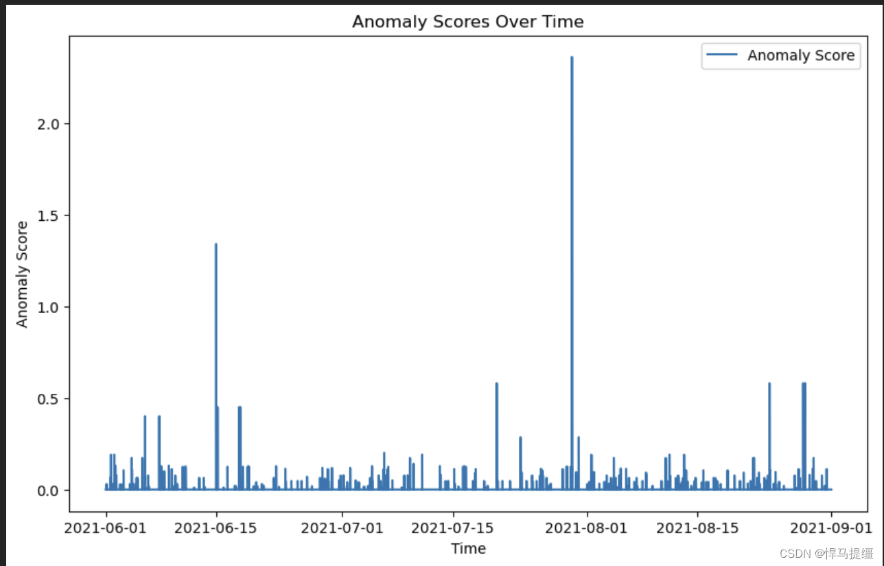

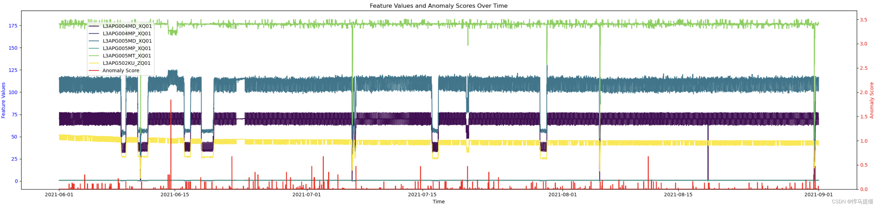
进一步可视化，方便做对比。