Lecture #14: Query Planning & Optimization

其实就是看官方笔记的时候整理了下重点或没那么容易理解的地方 

---

1. Overview

The DBMS needs to translate a SQL statement into an executable query plan.

The job of the DBMS’s optimizer is to pick an optimal plan for any given query.

There are two high-level strategies for query optimization:

• Use static rules, or heuristics.Heuristics match portions of the query with known patterns to assemble a plan,they never need to examine the data itself.

• Use cost-based search to read the data and estimate the cost of executing equivalent plans. The cost model chooses the plan with the lowest cost.

  

---

Logical vs. Physical Plans

The optimizer generates a mapping of a logical algebra expression to the optimal equivalent physical algebra expression. The logical plan is roughly equivalent to the relational algebra expressions in the query.

Physical operators define a specific execution strategy using an access path for the different operators in the query plan. Physical plans may depend on the physical format of the data that is processed (i.e. sorting, compression). 优化器的作用是将逻辑计划转换为最优的物理计划。

There does not always exist a one-to-one mapping from logical to physical plans.

---

2. Logical Query Optimization

Some selection optimizations include:

• Perform filters as early as possible (predicate pushdown).

• Reorder predicates so that the DBMS applies the most selective one first.
• Breakup a complex predicate and pushing it down (split conjunctive predicates)

Some projection optimizations include:

• Perform projections as early as possible to create smaller tuples and reduce intermediate results (projection pushdown).

• Project out all attributes except the ones requested or requires.

Some query rewrite optimizations include:

• Remove impossible or unnecessary predicates. In this optimization, the DBMS elides evaluation of predicates whose result does not change per tuple in a table Bypassing these predicates reduces computation cost.

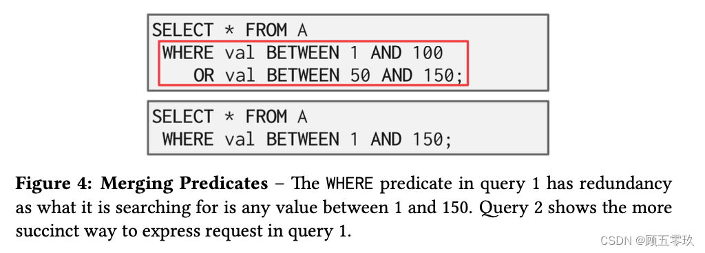
• Merging predicate as shown in Figure 4.

  

• Re-write the query by de-correlating and / or flattening nested subqueries. An example of this is shown in Figure 5.

The ordering of JOIN operations is a key determinant of query performance. Exhaustive enumeration of all possible join orders is inefficient, so join-ordering optimization requires a cost model. However, we can still eliminate unnecessary joins with a heuristic approach to optimization. An example of join elimination is shown in Figure 7.

---

3. Cost Estimations

DBMS’s use cost models to estimate the cost of executing a plan. These models evaluate equivalent plans for a query to help the DBMS select the most optimal one.

The cost of a query depends on several underlying metrics split between physical and logical costs, including:

• CPU: small cost, but tough to estimate.
• Disk I/O: the number of block transfers.块传输的数量
• Memory: the amount of DRAM used.内存成本
• Network: the number of messages sent.网络成本

Exhaustive enumeration of all valid plans for a query is much too slow for an optimizer to perform.

Optimizers must limit their search space in order to work efficiently.（限制搜索空间）

To approximate costs of queries, DBMS’s maintain internal statistics（内部统计信息） about tables, attributes, and indexes in their internal catalogs.

Most systems attempt to avoid on-the-fly computation （避免实时计算）by maintaining an internal table of statistics.

These internal tables may then be updated in the background.

For each relation R, the DBMS maintains the following information:

• $N_R$ : Number of tuples in $A$
• $V(A,R)$: Number of distinct values of attribute A

With the information listed above, the optimizer can derive the selection cardinality $SC(A,R)$ statistic. 选择基数，用来估计匹配某个属性值的记录数量。

The selection cardinality is the average number of records with a value for an attribute $A$ given $N_R/V(A,R)$ . 满足某个属性$A$的特定值的记录的平均数量

Note $V(A,R)$ that this assumes data uniformity. This assumption is often incorrect, but it simplifies the optimization process.(假设数据是均匀分布的，简化了优化过程)

---

Selection Statistics

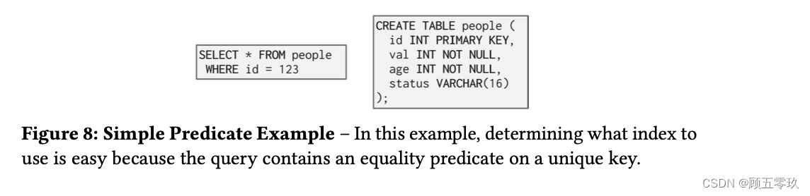
The selection cardinality can be used to determine the number of tuples that will be selected for a given input.

Equality predicates on unique keys are simple to estimate (see Figure 8). A more complex predicate is shown in Figure 9.

The selectivity (sel) （选择性）of a predicate P is the fraction of tuples that qualify. The formula used to compute selective depends on the type of predicate.

Selectivity for complex predicates is hard to estimate accurately which can pose a problem for certain systems. An example of a selectivity computation is shown in Figure 10.

Observe that the selectivity of a predicate is equivalent to the probability of that predicate. 可以通过概率的方法简化一些复杂选择性计算

This allows probability rules to be applied in many selectivity computations.

This is particularly useful when dealing with complex predicates.

For example, if we assume that multiple predicates involved in a conjunction are independent, we can compute the total selectivity of the conjunction as the product of the selectivities of the individual predicates.

---

Selectivity Computation Assumptions

In computing the selection cardinality of predicates, the following three assumptions are used.

• Uniform Data均匀数据假设: The distribution of values (except for the heavy hitters) is the same.
• Independent Predicates谓词独立性假设: The predicates on attributes are independent.
• Inclusion Principle包含原则: The domain of join keys overlap such that each key in the inner relation will also exist in the outer table.

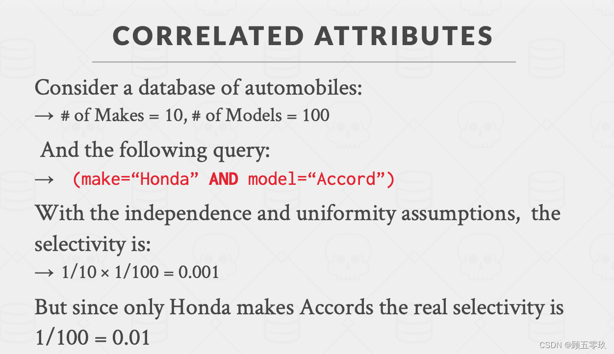
These assumptions are often not satisfied by real data. For example, correlated attributes break the assumption of independence of predicates.

---

4. Histograms直方图

Real data is often skewed and is tricky to make assumptions about.

However, storing every single value of a data set is expensive.

One way to reduce the amount of memory used by storing data in a histogram to group together values. An example of a graph with buckets is shown in Figure 11.

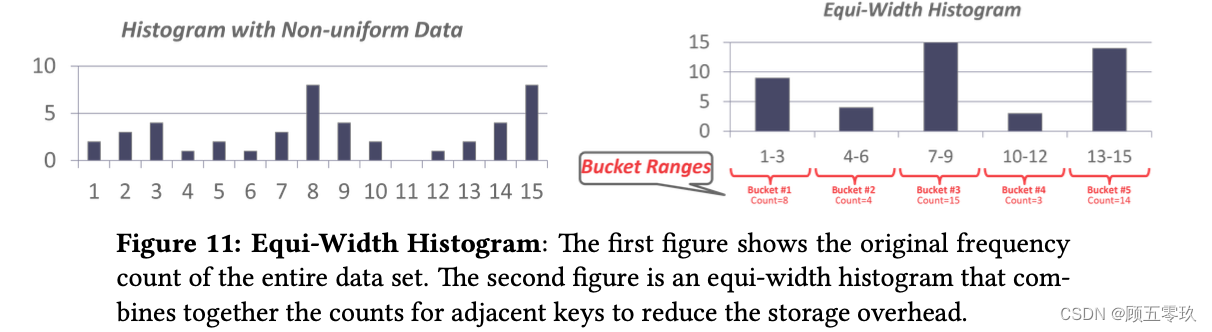
Another approach is to use a equi-depth histogram that varies the width of buckets so that the total number of occurrences for each bucket is roughly the same. An example is shown in Figure 12

In place of histograms, some systems may use sketches to generate approximate statistics about a data set.

---

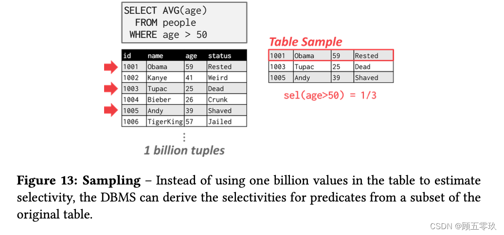
5. Sampling抽样

DBMS’s can use sampling to apply predicates to a smaller copy of the table with a similar distribution (see Figure 13).

The DBMS updates the sample whenever the amount of changes to the underlying table exceeds some threshold (e.g., 10% of the tuples).

---

6. Plan Enumeration枚举执行计划

After performing rule-based rewriting, the DBMS will enumerate different plans for the query and estimate their costs.

It then chooses the best plan for the query after exhausting all plans or some timeout.

---

7. Single-Relation Query Plans

For single-relation query plans, the biggest obstacle is choosing the best access method

• sequential scan,
• binary search,
• index scan, etc.

)Most new database systems just use heuristics, instead of a sophisticated cost model, to pick an access method. For OLTP queries, this is especially easy because they are sargable (Search Argument Able), which means that there exists a best index that can be selected for the query. This can also be implemented with simple heuristics.

---

8. Multi-Relation Query Plans

For Multi-Relation query plans, as number of joins increases, the number of alternative plans grow rapidly. Consequently, it is important to restrict the search space so as to be able to find the optimal plan in a reasonable amount of time.

There are two ways to approach this search problem:

• Bottom-up: Start with nothing and then build up the plan to get to the outcome that you want.从零开始后构建计划
  • Examples: IBM System R, DB2, MySQL, Postgres, most open-source DBMSs.
• Top-down: Start with the outcome that you want, and then work down the tree to find the optimal从想要的结果开始，沿着树向下工作 plan that gets you to that goal.
  • Examples: MSSQL, Greenplum, CockroachDB, Volcano。

---

9. Bottom-up optimization example - System R

Use static rules to perform initial optimization. Then use dynamic programming to determine the best join order for tables using a divide-and conquer search method.

• Break query up into blocks and generate the logical operators for each block
• For each logical operator, generate a set of physical operators that implement it
• Then, iteratively construct a ”left-deep”tree that minimizes the estimated amount of work to execute the plan

---

10. Top-down optimization example - Volcano

Start with a logical plan of what we want the query to be. Perform a branch-and-bound search to traverse the plan tree by converting logical operators into physical operators.

• Keep track of global best plan during search.
• Treat physical properties of data as first-class entities during planning.

---