


Precision_Agriculture是一个用于计算遥感光谱参数的开源平台,这里梳理了一点功能,由于采用的图像仅为示例图像,大家可以根据自己的需求自行调整,错误之处敬请包含谅解。
源码地址: Precision_Agriculture/README.md at master · px39n/Precision_Agriculture · GitHub
README
Model Precision_Agriculture
SUMMARY
遥感的目标之一是能够在最短的时间内提供有用的信息,供决策之用。因此,遥感被认为是精准农业的基本工具,因为它可以对作物的整个生长期进行监测,及时提供诊断评估信息。这项任务必须找出限制作物生长的因素,并及时决定是否进行农艺干预。
一种很有前景的方法是整合从时间、镶嵌、多光谱和热成像中获得的数据。通过这两种方法,我们可以获得以下产品: 这些产品使我们能够识别压力区,为农业管理任务提供支持。
因此,我们的目标是开发一个开源平台,该平台发布在 GitHub 平台上,能够通过处理无人机拍摄的图像,捕捉植物在不同生长阶段的反射率变化,从而生成诊断工具,或对水分胁迫、健康状况(病虫害侵袭)、物候状态、营养缺乏、生产力和性能等发出预警。
关键词:植被指数、物候状态、农业管理、开源平台。
INTRODUCTION
在生物物理参数中,可通过植被指数确定的最重要参数是:叶片的叶绿素含量(Chl)、叶面积指数(LAI)和湿度。
叶绿素含量(Chl)是植被进行光合作用能力的指标,光合作用是植物生长和生存的基本过程,也与植物吸收大气中二氧化碳的能力直接相关。
叶面积指数(LAI)的定义是单位面积土壤中单侧叶片的面积,它提供了植物冠层的信息,是气候、农艺和生态研究的基本参数。
湿度是植物生理阶段(健康状况和物候)的其他生物指标。植物需要一定量的水分来进行蒸腾和其他过程。蒸腾作用是通过称为气孔的微小叶片开口将水分排入大气的过程。植物在生长过程中会出现两种现象:张力和质解。细胞膨胀是细胞膨胀或充满水分的现象,而细胞溶解则是相反的过程,细胞在枯萎时会自然失水。在许多情况下,植被对疾病或水胁迫等外部侵害的反应是提高温度。基于高分辨率热图像的新型遥感方法已经证明了其在检测水分胁迫和通过检测植被发出的荧光和叶绿素活性估算光合作用性能方面的潜力。
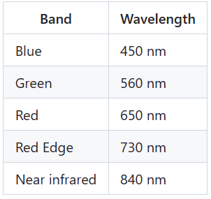
如今,无人驾驶飞行器上的相机传感器可以捕捉红色、红边、近红外和热波段的光谱(表 1)。
表1:可用的多光谱波段(Multispectral bands)波长。
Multispectral bands
Vegetation index calculations(植被指数计算)
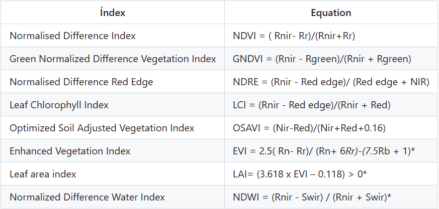
根据这些波长可生成以下光谱指数(表 2)。
表 2:根据无人机上相机的可用波长生成的光谱指数。
定义植物健康状况标签
|
| NDVI 1 | NDVI 1 < NDVI 2 |
| 等级 | 描述 | 描述 |
| -1 to 0 | 水、裸土 | 水、裸土 |
| 0 to 0.15 | 植被稀疏或作物处于生长初期的土壤(发芽) | 活力差、植株弱 |
| 0.15 to 0.30 | 处于中间发育阶段的植物( 长叶) | 花叶比例失调 |
| 0.30 to 0.45 | 处于中间发育阶段的植物 (长叶) | 花果比例失调;果实含糖量低,果实缺乏色泽,果实品质差 |
| 0.45 to 0.60 | 处于成株期或成熟期的植物( 结果) | 花果比例失调;果实含糖量低,果实缺乏色泽,果实品质差 |
| 0.60 to >0.80 | 处于成株期或成熟期的植株 (果实成熟) | 花果比例失调;果实含糖量低,果实缺乏色泽,果实品质差 |
该解决方案的局限性
1.在使用该工具之前,必须构建多光谱正射影像图;
2. RGB 波段分段处理;
3.必须知道您将使用的波段格式以及每张图像的元数据(tiff、GeoTiff);
4.在这种情况下,方法和支持仅适用于 Phantom 4 RTK 多光谱用户;
TO DO LIST
在开发这项工作时,我们遵循以下清单:
- Mosaico vegetation index(Mosaico植被指数)
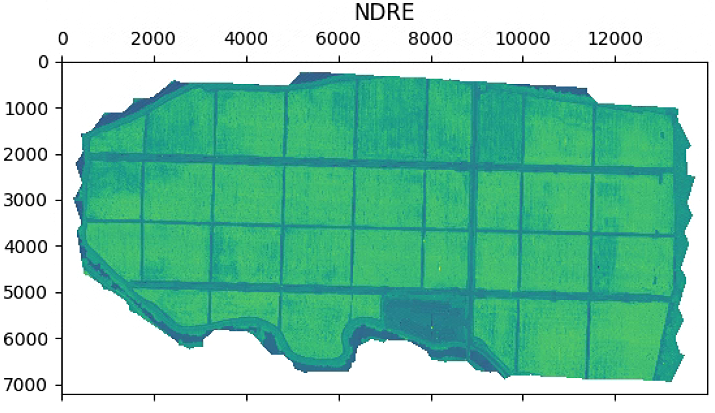
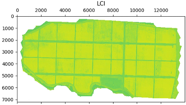
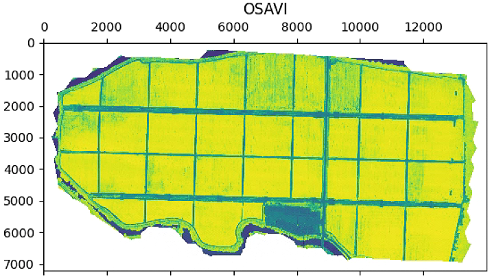
1- NDVI;2- GNDVI;3- NDRE;4- LCI;5- OSAVI
- 葡萄园
- 草场
- 其他作物
-Labelin
1- Weed detection;2- Disease detection
- 葡萄园
- 草场
- 其他作物
代码梳理
Caso2.py
'''
复现者备注, 本项目中包含大量R语言函数包, 已尽可能做注释
'''
# 导包
import numpy as np
from skimage import io
from veg_index import Image_Multi
import matplotlib.pyplot as plt
from matplotlib import path
import georasters as gr # georasters 使用地理信息栅格的工具
import cv2
# import matplotlib
# matplotlib.use('TkAgg')
# 功能模块
def aux_index(Im):
Im.raster = Im.raster[0, :, :] # raster,栅格函数
Im.shape = Im.raster.shape
return Im
def ImRGBN2Split(ImRGBN, indx): # 这个函数要根据图像来分离RGB通道,因此需要自己调试index
proj = ImRGBN.projection # projection投影,投影转换是将栅格对象的投影由一种转换到另一种
nodata = ImRGBN.nodata_value # 栅格数据中的NoData数值
datatype = ImRGBN.datatype
geot = ImRGBN.geot
return gr.GeoRaster(ImRGBN.raster[indx, :, :], geot, nodata, proj, datatype)
# 读图
# path_im = 'Caso2/banano_rgb_1.tif'
path_im = 'Caso2/result.tif' # RGB TIF图路径
ImRGBN = gr.from_file(path_im) # from_fil函数,Create a GeoRaster object from a file
# print(ImRGBN.shape) # (4, 7209, 13994) 可以看到RGBN只有四个通道
'''
# 备注, 这一块是为了测试veg_index.py中的RGBN图像通道分离功能,不是源码中的
im_red = ImRGBN2Split(ImRGBN, 0) # type(im_red.raster) <class 'numpy.ma.core.MaskedArray'> im_red.sum()=7166081056
# print(im_red, im_red.nodata_value, im_red.shape, type(im_red.shape)) # <georasters.georasters.GeoRaster object at 0x7fea43106880> 0.0 (7209, 13994) <class 'tuple'>
# arr = np.uint8(np.isnan(im_red.raster)) # 这也是空的<class 'numpy.ma.core.MaskedArray'> arr.sum()=0
# countours, hierarchy = cv2.findContours(np.uint8(np.isnan(im_red.raster)), cv2.RETR_TREE, cv2.CHAIN_APPROX_SIMPLE)
countours, hierarchy = cv2.findContours(np.uint8(im_red.raster), cv2.RETR_TREE, cv2.CHAIN_APPROX_SIMPLE)
# cv2.findContours(image, mode, method) mode:轮廓的模式, cv2.RETR_TREE,建立一个等级树结构的轮廓。method, 轮廓的近似方法,cv2.CHAIN_APPROX_SIMPLE压缩水平方向,垂直方向,对角线方向的元素
print(countours, type(countours)) # 看看找没找到边界
print([ctln.shape[0] for ctln in countours]) # 看看是不是空列表
'''
# 波段最小值
im_multi = Image_Multi()
im_multi.load_images(im_red = ImRGBN2Split(ImRGBN, 0), im_green = ImRGBN2Split(ImRGBN, 1),
im_blue = ImRGBN2Split(ImRGBN, 2),im_nir = ImRGBN2Split(ImRGBN, 3),
im_rededge = ImRGBN2Split(ImRGBN, 3))
# Nir = Rededge
# print(ImRGBN.min()) # 1
# print(im_multi.im_red.min()) # 1
# print(im_multi.im_green.min()) # 1
# print(im_multi.im_blue.min()) # 1
# print(im_multi.im_nir.min()) # 1
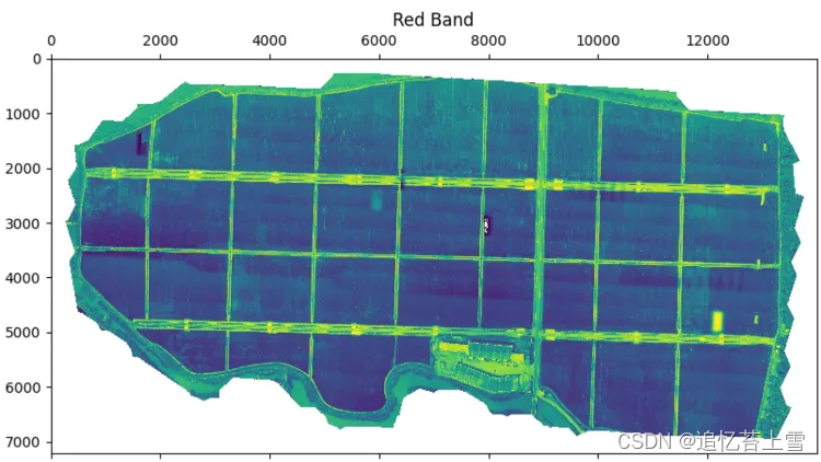
# 分离各波段图像
plt.figure(figsize=(15, 15))
im_multi.im_red.plot()
plt.title('Red Band')
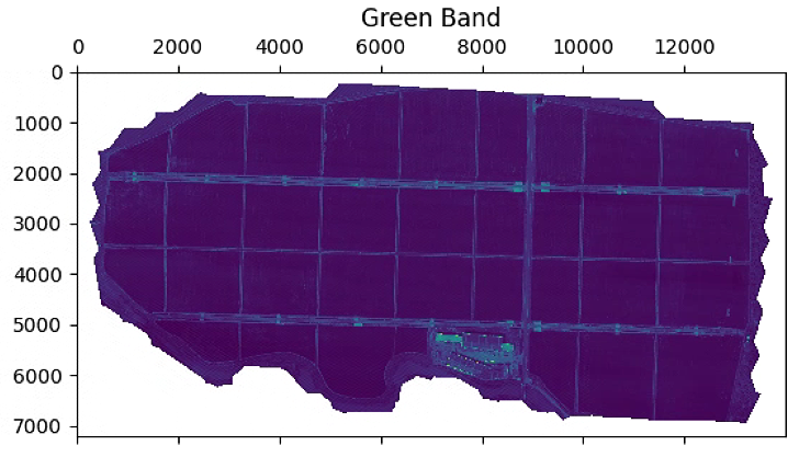
plt.figure(figsize=(15, 15))
im_multi.im_green.plot()
plt.title('Green Band')
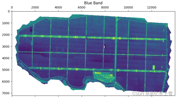
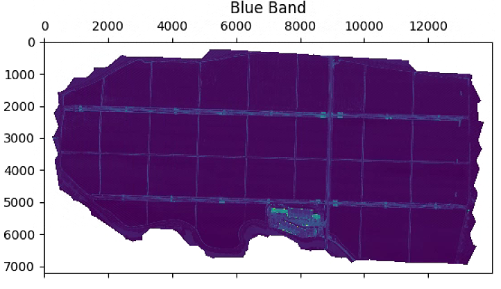
plt.figure(figsize=(15, 15))
im_multi.im_blue.plot()
plt.title('Blue Band')
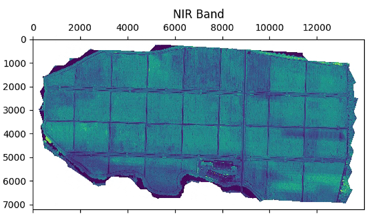
plt.figure(figsize=(15, 15))
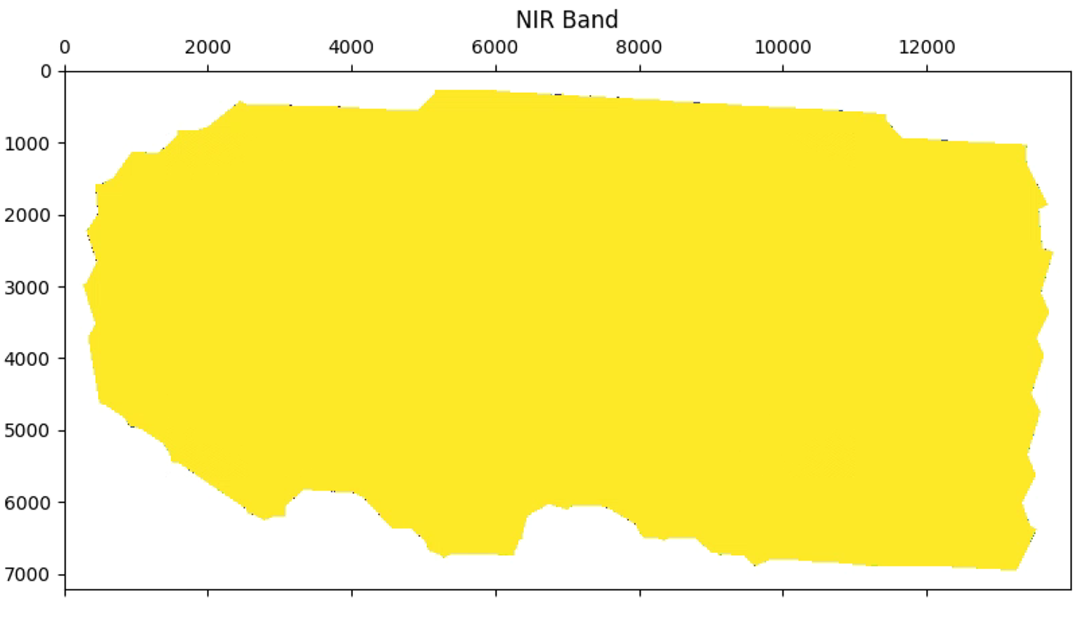
im_multi.im_nir.plot()
plt.title('NIR Band')
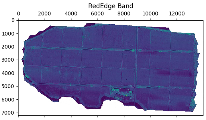
plt.figure(figsize=(15, 15))
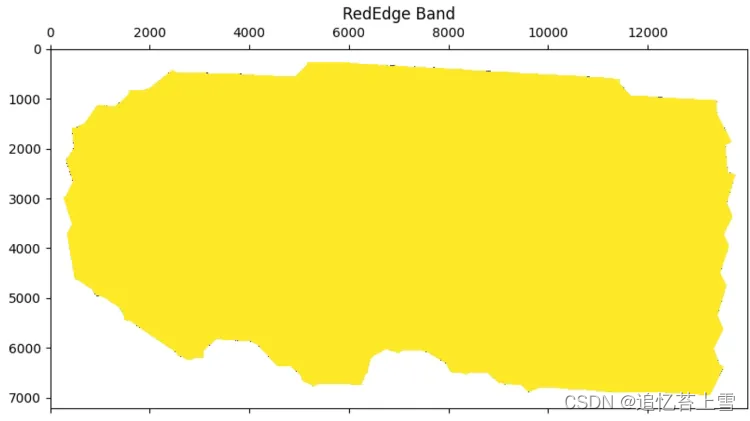
im_multi.im_rededge.plot()
plt.title('RedEdge Band')
plt.show()结果如下

# 植被指数可视化
plt.figure(figsize=(15, 15))
aux =im_multi.NDVI().raster
aux[aux>20] = 20
plt.imshow(aux)
plt.title('NDVI')
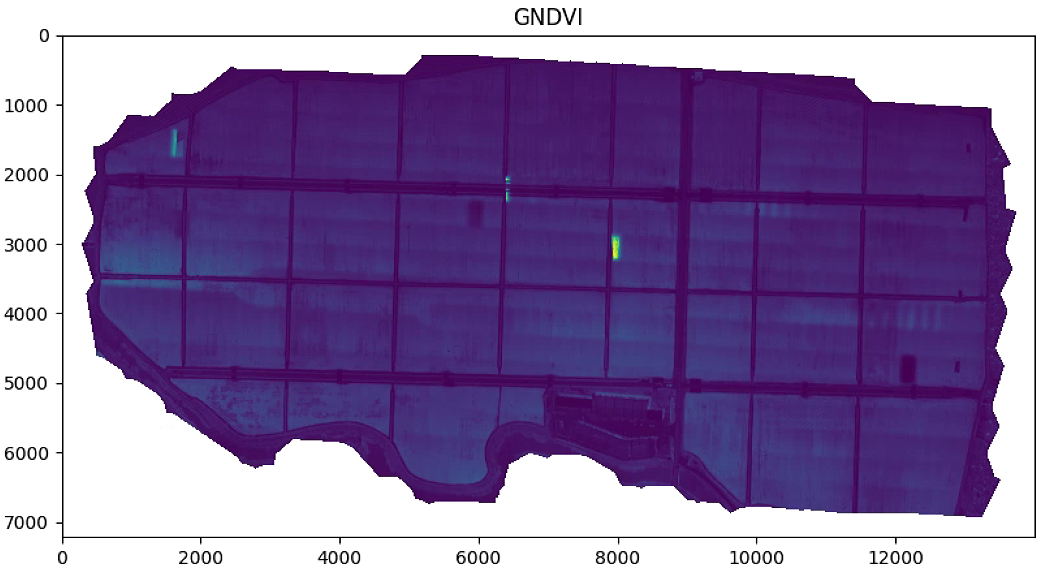
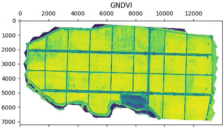
plt.figure(figsize=(15, 15))
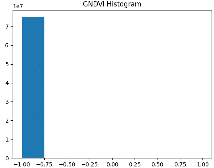
aux =im_multi.GNDVI().raster
aux[aux>20] = 20
plt.imshow(aux)
plt.title('GNDVI')
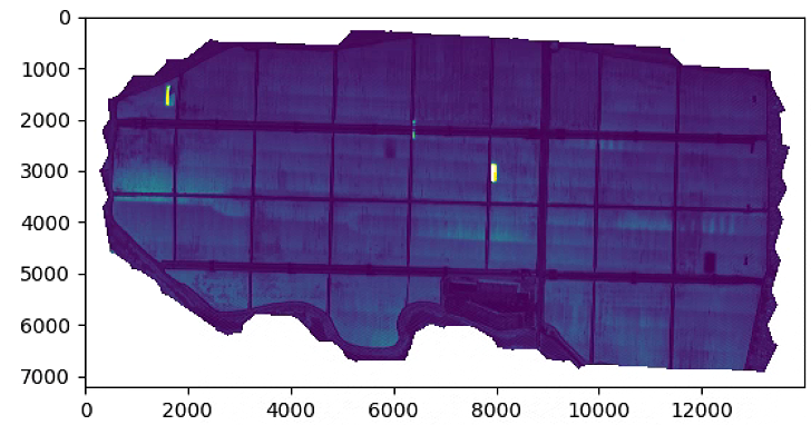
plt.figure(figsize=(15, 15))
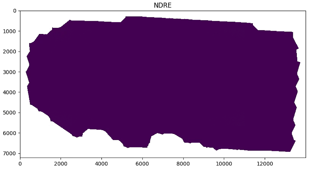
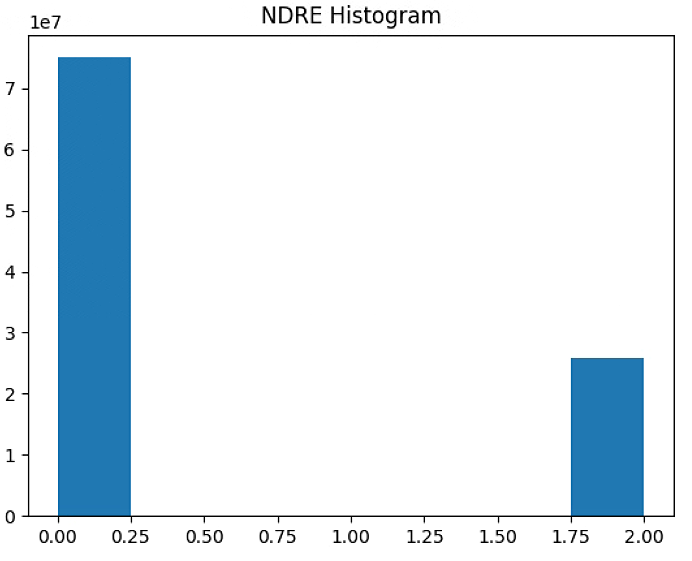
aux =im_multi.NDRE().raster
aux[aux>20] = 20
plt.imshow(aux)
plt.title('NDRE')
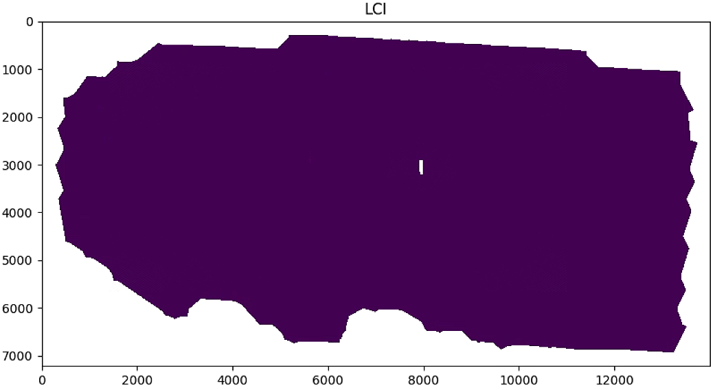
plt.figure(figsize=(15, 15))
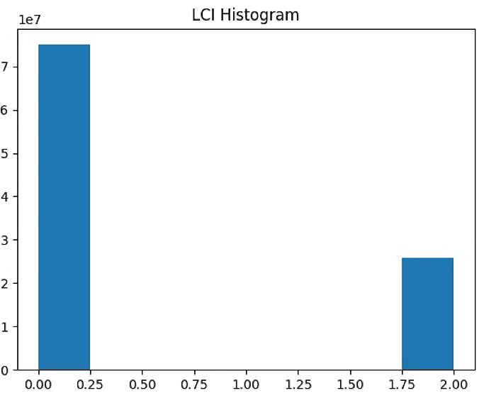
aux =im_multi.LCI().raster
aux[aux>20] = 20
plt.imshow(aux)
plt.title('LCI')
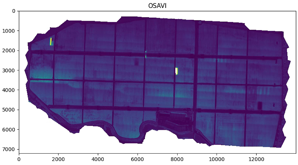
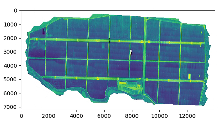
plt.figure(figsize=(15, 15))
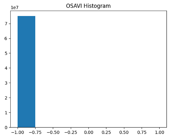
aux =im_multi.OSAVI().raster
aux[aux>20] = 20
plt.imshow(aux)
plt.title('OSAVI')
plt.show()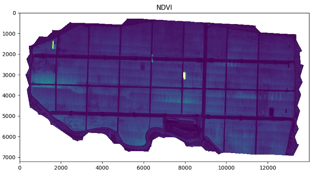
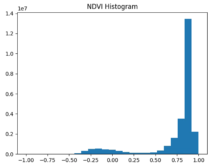
# 直方图
n_bins = 8
plt.figure(1)
NDVI_raster = im_multi.NDVI().raster
NDVI_raster[NDVI_raster > 255] = 255
NDVI_raster = 2. * (NDVI_raster - np.ma.min(NDVI_raster)) / np.ma.ptp(NDVI_raster) - 1
plt.hist(NDVI_raster[~np.isnan(NDVI_raster)], bins = n_bins)
plt.title('NDVI Histogram')
#plt.savefig('Barrack A/NDVI_Histogram_'+ str(n_bins))
plt.figure(2)
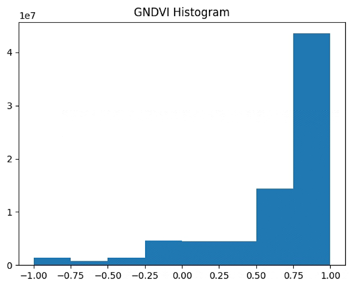
GNDVI_raster = im_multi.GNDVI().raster
GNDVI_raster[GNDVI_raster > 255] = 255
GNDVI_raster = 2. * (GNDVI_raster - np.ma.min(GNDVI_raster)) / np.ma.ptp(GNDVI_raster) - 1
plt.hist(GNDVI_raster[~np.isnan(GNDVI_raster)], bins = n_bins)
plt.title('GNDVI Histogram')
#plt.savefig('Barrack A/GNDVI_Histogram_'+ str(n_bins))
plt.figure(3)
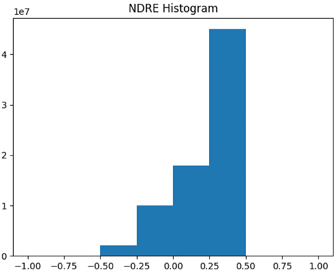
NDRE_raster = im_multi.NDRE().raster
NDRE_raster[NDRE_raster > 255] = 255
NDRE_raster = 2. * (NDRE_raster - np.ma.min(NDRE_raster)) / np.ma.ptp(NDRE_raster) - 1
plt.hist(NDRE_raster[~np.isnan(NDRE_raster)], bins = n_bins)
plt.title('NDRE Histogram')
#plt.savefig('Barrack A/NDRE_Histogram_'+ str(n_bins))
plt.figure(4)
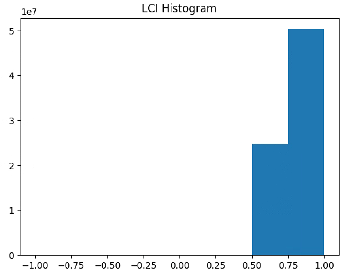
LCI_raster = im_multi.LCI().raster
LCI_raster[LCI_raster > 255] = 255
LCI_raster = 2. * (LCI_raster - np.ma.min(LCI_raster)) / np.ma.ptp(LCI_raster) - 1
plt.hist(LCI_raster[~np.isnan(LCI_raster)], bins = n_bins)
plt.title('LCI Histogram')
#plt.savefig('Barrack A/LCI_Histogram_'+ str(n_bins))
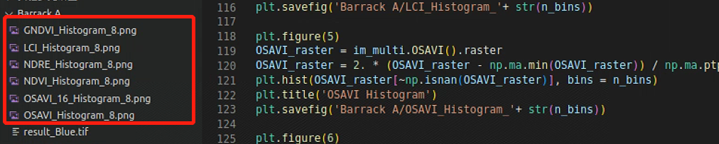
plt.figure(5)
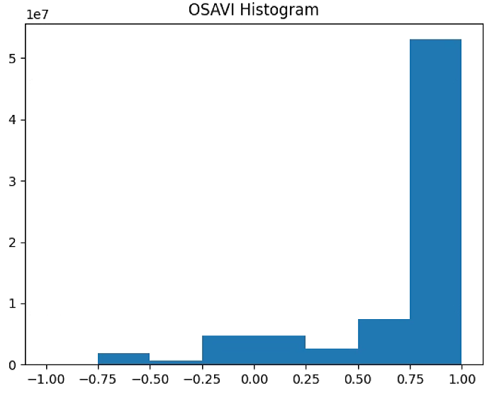
OSAVI_raster = im_multi.OSAVI().raster
OSAVI_raster[OSAVI_raster > 255] = 255
OSAVI_raster = 2. * (OSAVI_raster - np.ma.min(OSAVI_raster)) / np.ma.ptp(OSAVI_raster) - 1
plt.hist(OSAVI_raster[~np.isnan(OSAVI_raster)], bins = n_bins)
plt.title('OSAVI Histogram')
#plt.savefig('Barrack A/OSAVI_Histogram_'+ str(n_bins))
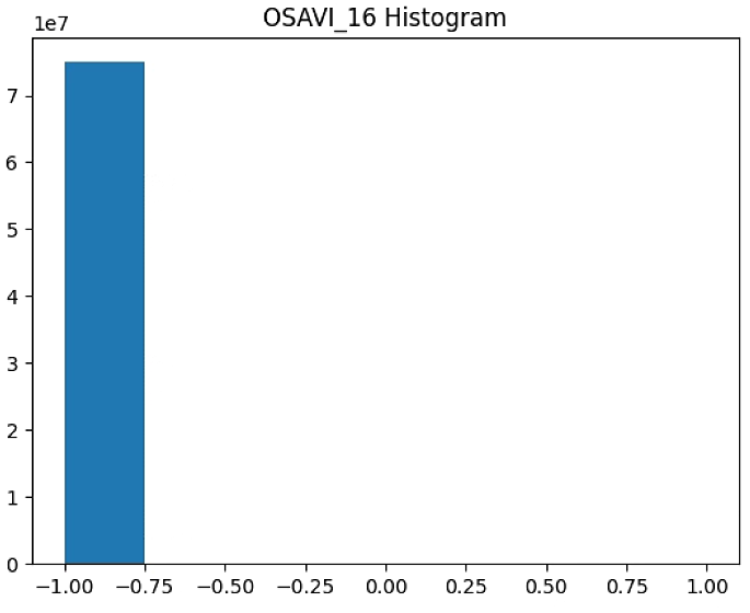
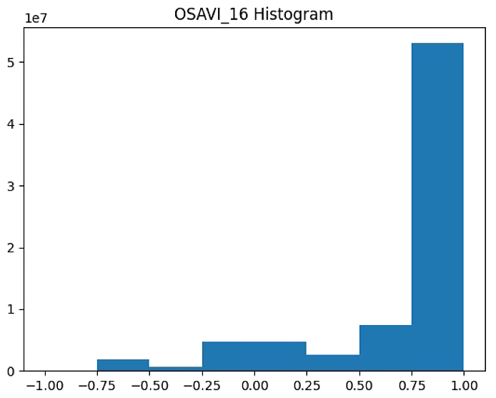
plt.figure(6)
OSAVI_raster = im_multi.OSAVI_16().raster
OSAVI_raster[OSAVI_raster > 255] = 255
OSAVI_raster = 2. * (OSAVI_raster - np.ma.min(OSAVI_raster)) / np.ma.ptp(OSAVI_raster) - 1
plt.hist(OSAVI_raster[~np.isnan(OSAVI_raster)], bins = n_bins)
plt.title('OSAVI_16 Histogram')
#plt.savefig('Barrack A/OSAVI_16_Histogram_'+ str(n_bins))
plt.show()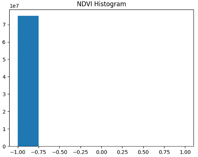
# A1, A2, NDVI
RED = im_multi.im_red.raster
NIR = im_multi.im_nir.raster
A1 = NIR-RED
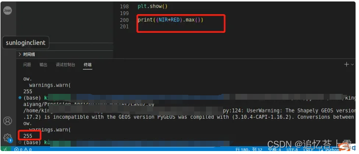
A2 = NIR+RED
NDVI = A1/(A2 + .01)
NDVI[NDVI>20] = 20
plt.figure(1)
plt.imshow(A1)
plt.figure(2)
plt.imshow(A2)
plt.figure(3)
plt.imshow(NDVI)
# plt.show()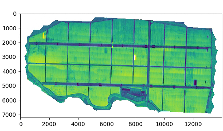
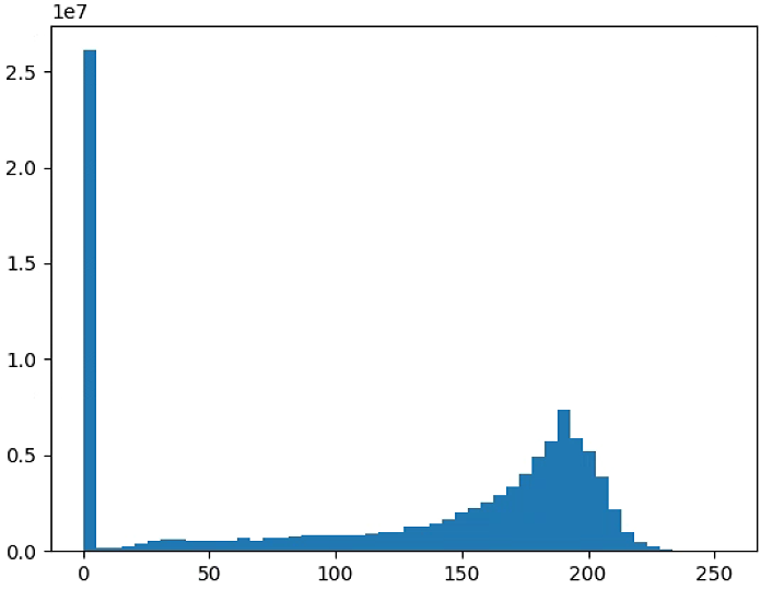
# 直方图
n_bins = 50
plt.figure(2)
NDVI_raster = (NIR-RED)#/(NIR+RED+ 0.001)
#NDVI_raster[NDVI_raster > 255] = 255
#NDVI_raster = 2. * (NDVI_raster - np.ma.min(NDVI_raster)) / np.ma.ptp(NDVI_raster) - 1
plt.hist(NDVI_raster[~np.isnan(NDVI_raster)], bins = n_bins)
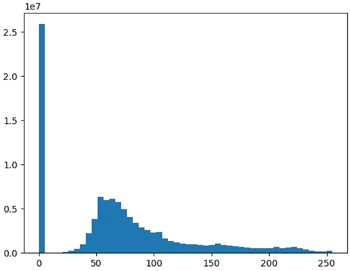
plt.figure(3)
NDVI_raster = (NIR+RED)#/(NIR+RED+ 0.001)
#NDVI_raster[NDVI_raster > 255] = 255
#NDVI_raster = 2. * (NDVI_raster - np.ma.min(NDVI_raster)) / np.ma.ptp(NDVI_raster) - 1
plt.hist(NDVI_raster[~np.isnan(NDVI_raster)], bins = n_bins)
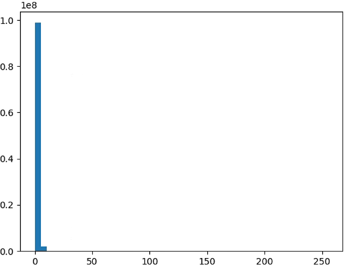
plt.figure(4)
NDVI_raster = np.uint8(NIR-RED)/(NIR+RED+ 0.001)
NDVI_raster[NDVI_raster > 255] = 255
#NDVI_raster = 2. * (NDVI_raster - np.ma.min(NDVI_raster)) / np.ma.ptp(NDVI_raster) - 1
plt.hist(NDVI_raster[~np.isnan(NDVI_raster)], bins = n_bins)
 Circle_Analysis.py
# 导包
import numpy as np
from veg_index import Image_Multi
import matplotlib.pyplot as plt
from matplotlib import path
import matplotlib.patches as patches
from skimage import draw
import scipy.ndimage as ndimage
import Utils
import cv2
import matplotlib as mpl
# 加载图像
path_barrack = "Barrack B/"
im_red_path = path_barrack + "result_Red.tif"
im_green_path = path_barrack + "result_Green.tif"
im_blue_path = path_barrack + "result_Blue.tif"
im_nir_path = path_barrack + "result_NIR.tif"
im_rededge_path = path_barrack + "result_RedEdge.tif"
im_multi = Image_Multi(im_red_path, im_green_path, im_blue_path, im_nir_path, im_rededge_path)
#### Polygon Barrack A ##############
#List_P = [(1600, 500),(4800, 3600), (1100, 1900), (5500, 1900)]
#List_P = [(500, 3700), (1000, 1900), (4900, 3600), (4000, 5500)]
#### Polygon Barrack B ##############
#List_P = [(850, 150),(5500, 1800), (4900, 3500), (300, 1800)]
List_P = [(300, 1800), (4900, 3500), (4500, 5300), (10, 3600)]
im_multi_seg = im_multi.Segmentation(List_P)
plt.figure(0)
plt.figure(figsize=(16, 16))
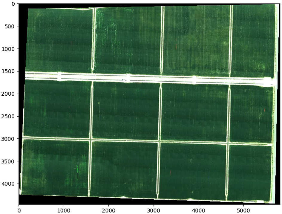
plt.imshow(im_multi.RGB().raster.copy())
plt.title('Subdive Origin Image')
ax = plt.gca()
for i,Poly in enumerate([List_P]):
poly = patches.Polygon(Poly,
linewidth=2,
edgecolor='red',
fill = False)
plt.text(np.mean([x[0] for x in Poly]), np.mean([y[1] for y in Poly]) , str(i), bbox=dict(facecolor='red', alpha=0.8))
ax.add_patch(poly)
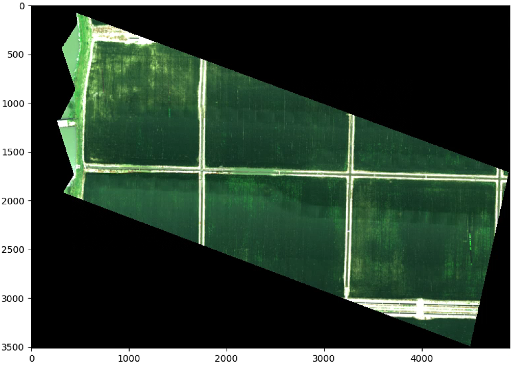
plt.figure(1)
plt.figure(figsize=(16, 16))
plt.imshow(im_multi_seg.RGB().raster)
plt。show()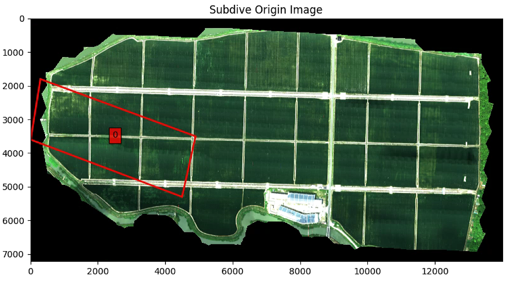
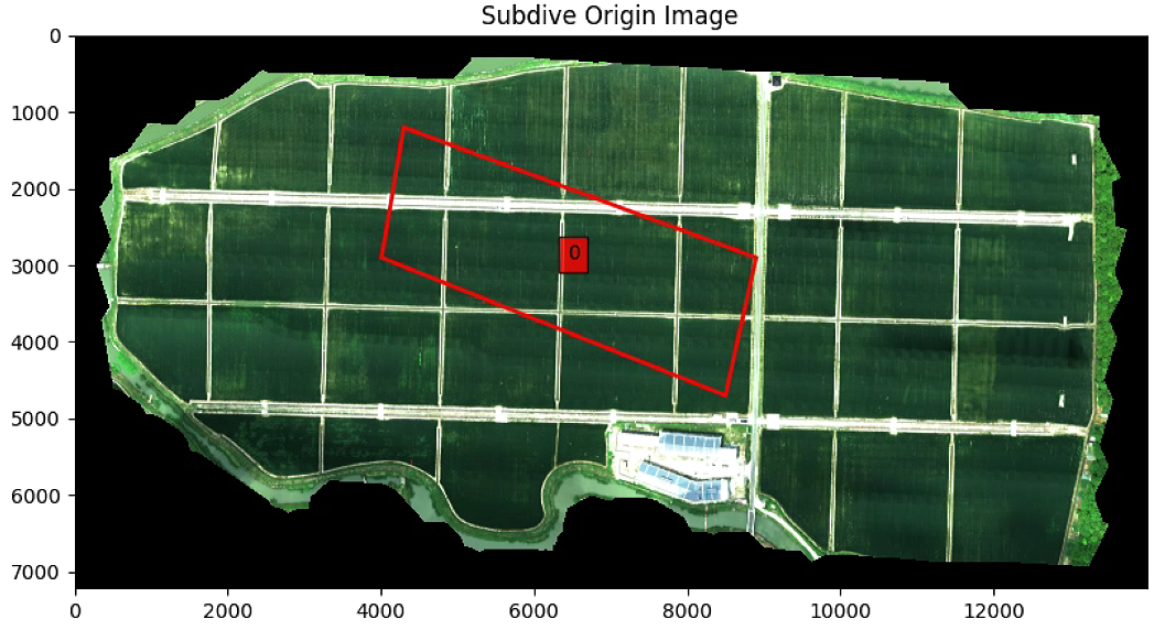
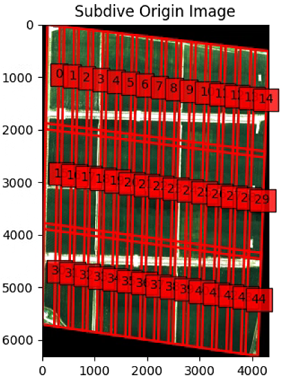
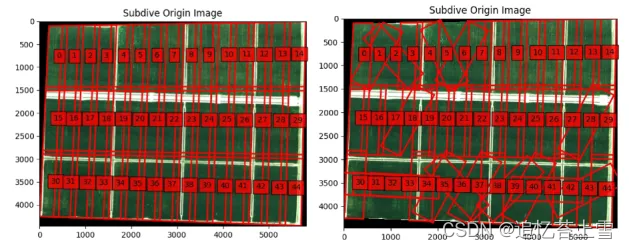
要是改List_P (List_P顺时针从上到下)
![]()
则输出为
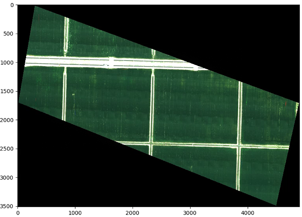
# 分割图像
split_Weight, split_Height = 15, 3
overlap = 0.01
List_subdivide = im_multi_seg.subdivision_rect(split_Weight, split_Height, overlap)
List_subdivide_correct = im_multi_seg.correction_subimage(List_subdivide)
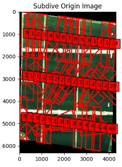
plt.figure(0)
plt.imshow(im_multi_seg.RGB().raster.copy())
plt.title('Subdive Origin Image')
ax = plt.gca()
for i,Poly in enumerate(List_subdivide):
poly = patches.Polygon(Poly,
linewidth=2,
edgecolor='red',
fill = False)
plt.text(np.mean([x[0] for x in Poly]), np.mean([y[1] for y in Poly]) , str(i), bbox=dict(facecolor='red', alpha=0.8))
ax.add_patch(poly)
plt.figure(1)
plt.imshow(im_multi_seg.RGB().raster.copy())
plt.title('Subdive Origin Image')
ax = plt.gca()
for i,Poly in enumerate(List_subdivide_correct):
poly = patches.Polygon(Poly,
linewidth=2,
edgecolor='red',
fill = False)
plt.text(np.mean([x[0] for x in Poly]), np.mean([y[1] for y in Poly]) , str(i), bbox=dict(facecolor='red', alpha=0.8))
ax.add_patch(poly)
plt.show()这一块有一个报错,强制转了一下类型
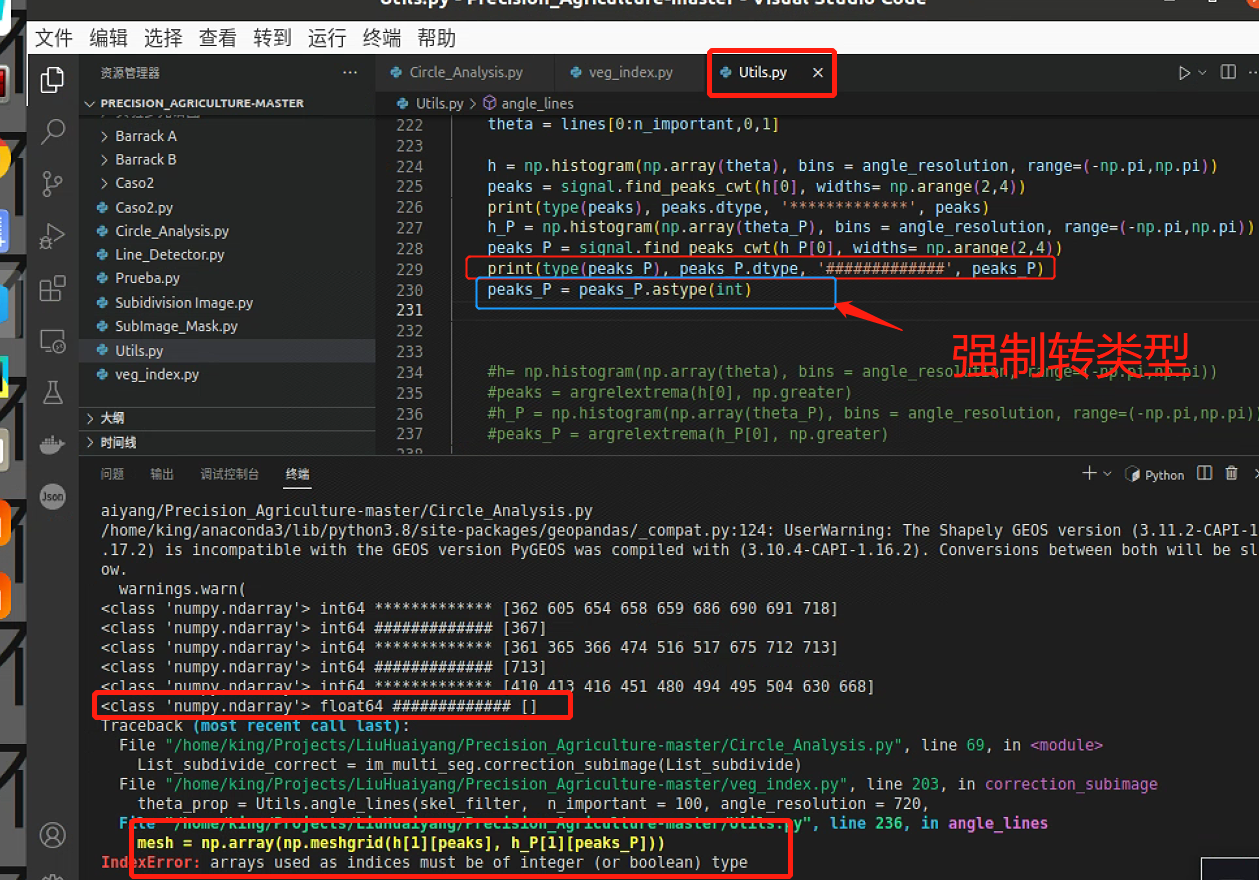
但是寻找峰值的时候出现了空列表,这是因为峰值左右有相同的两个点,导致寻不到,后面计算最小索引会报空列表的错
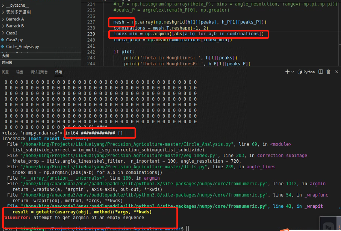
所以需要调一下参数
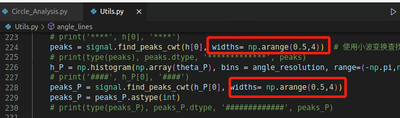
输出得到
# 直线检测
th_NDVI = 0.3
vertical_kernel_size_h = 10
vertical_kernel_size_w = 5
th_small_areas = 30
lines_width = 1
merge_bt_line = 10
List_lines_origin_complete = im_multi_seg.detector_lines(List_subdivide_correct,
th_NDVI,
vertical_kernel_size_h,
vertical_kernel_size_w,
th_small_areas,
lines_width,
merge_bt_line)
plt.figure(0)
plt.figure(figsize=(16, 16))
plt.imshow(im_multi_seg.RGB().raster)
ax = plt.gca()
for i,Poly in enumerate(List_lines_origin_complete):
poly = patches.Polygon(Poly,
linewidth=2,
edgecolor='red',
alpha=0.5,
fill = True)
plt.text(np.mean([x[0] for x in Poly]), np.mean([y[1] for y in Poly]) , str(i), bbox=dict(facecolor='red', alpha=0.8))
ax.add_patch(poly)
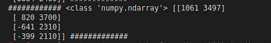
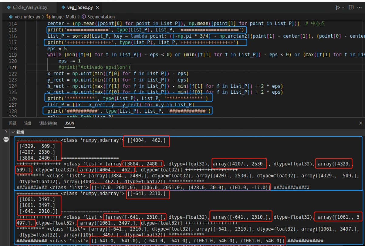
plt.show()其中遭遇过如下报错,说明遇到数据类型混合了
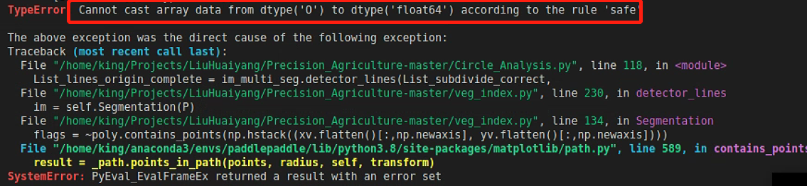
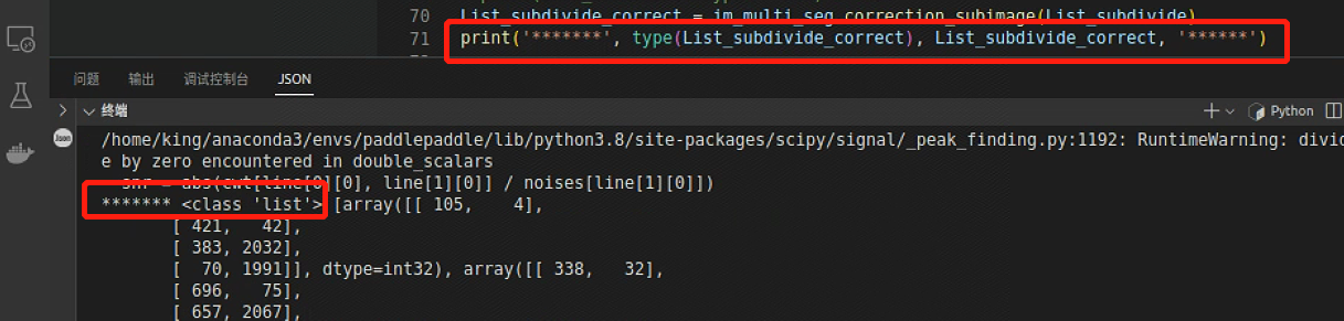
打印报错数据类型,是所需的List没有错
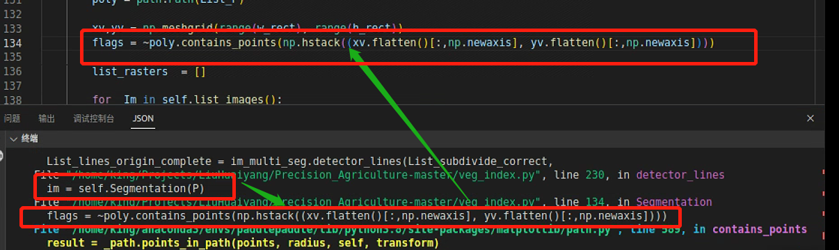
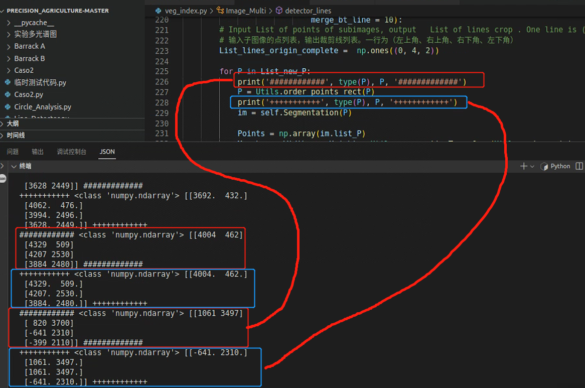
跳转到报错处
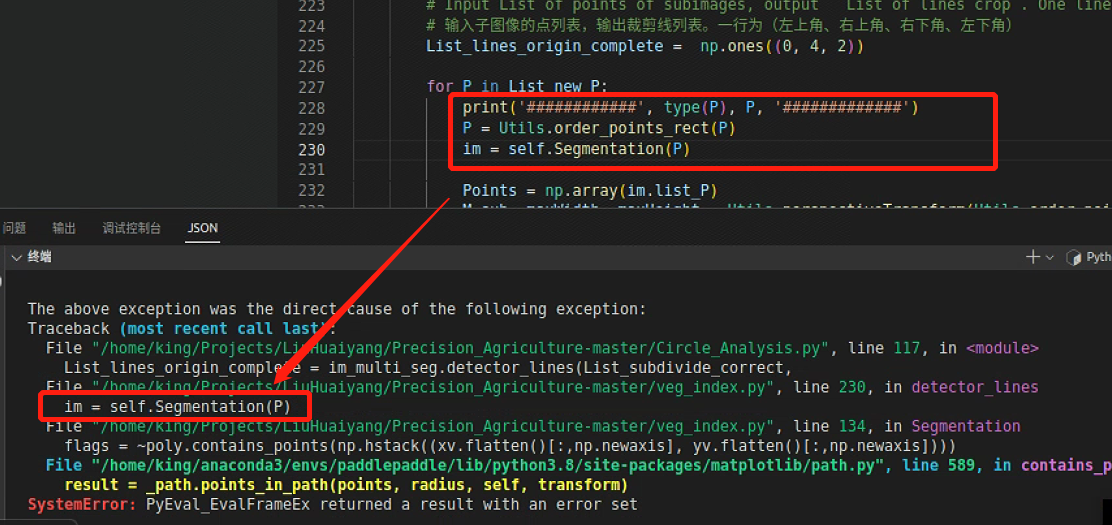
打印一下P的类型和数据,发现List中的多维数组读取到中间就断掉了
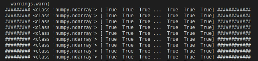
跳到下一处报错
打印输出flags,发现是由bool数组成的数组,这是没有数据类型混合的,而且也没有输出完整,说明是有数据影响到了flags输出
进一步发现导致path报错的是List_P
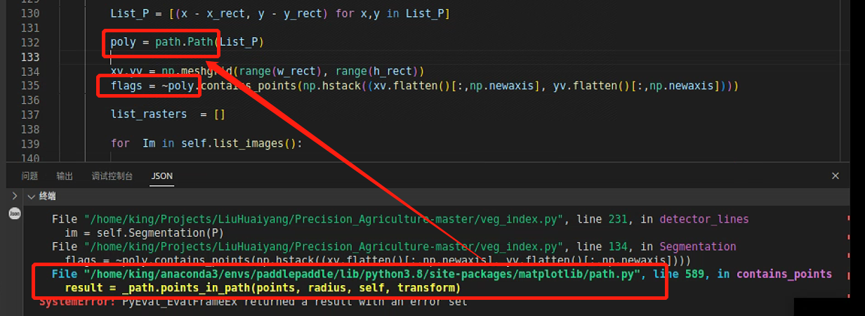
输出一下List_P,发现问题了,有一组数据,组不成矩形,就是上面断掉的数据
继续回到这一处报错,看看是不是因为P的排序出问题
果然是排序出了问题,跳到排序函数
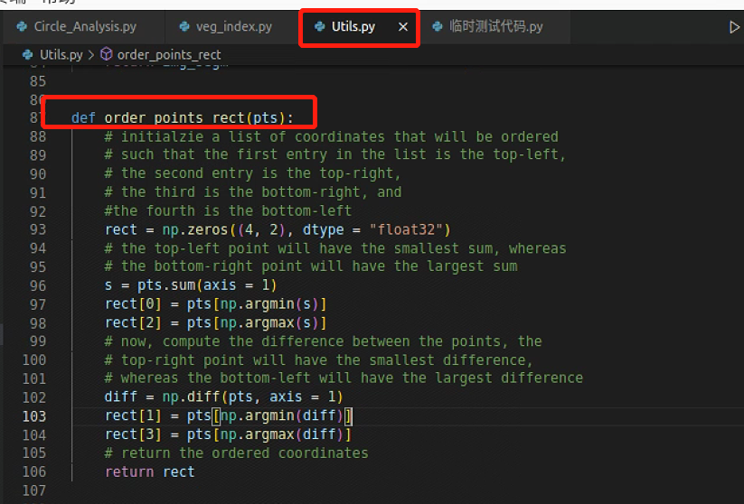
将有问题的数组拉出来重新排序,发现问题了

重新选定区域分割,发现可以了,这应该是数据的问题,按照上一步重新选定分割区域
可以输出了
# Put Circle on lines

r_circle = 10
centers_circles = Utils.lines2circles(List_lines_origin_complete, r_circle)

#### Save Result###########
np.save('Barrack A/centers_circles.npy', centers_circles)
#centers_circles = np.load('Barrack A/centers_circles.npy')


plt.figure(0)
plt.figure(figsize=(16, 16))
plt.imshow(im_multi_seg.RGB().raster)

ax = plt.gca()


for x1, y1 in centers_circles[:,:]:
    circle = patches.Circle((x1, y1), r_circle,
                            linewidth=2,
                             edgecolor='blue',
                             alpha=0.5,
                             fill = True)
    ax.add_patch(circle)
plt.show()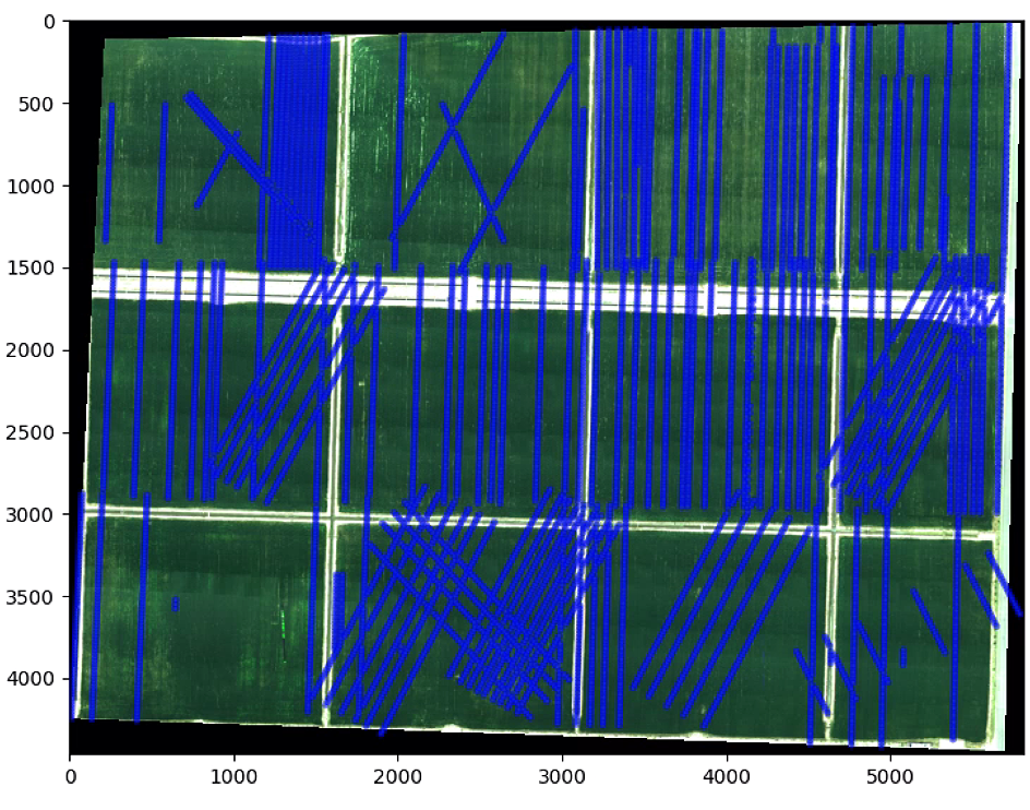
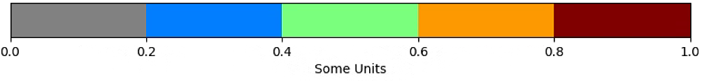
# The color of the circle depends on the NDVI
r_circle = 10
NDVI = im_multi_seg.NDVI().raster
NDVI_circle_index = []
for c in centers_circles:
rr, cc = draw.disk((c[1], c[0]), radius=r_circle, shape=NDVI.shape)
NDVI_circle_index.append(np.mean(NDVI[rr, cc]))
NDVI_circle_index = np.array(NDVI_circle_index)
n_color = 5
# create the new map
cmap = plt.cm.jet # define the colormap
# extract all colors from the .jet map
cmaplist = [cmap(i) for i in range(cmap.N)]
# force the first color entry to be grey
cmaplist[0] = (.5, .5, .5, 1.0)
cmap = mpl.colors.LinearSegmentedColormap.from_list('Custom cmap', cmaplist, cmap.N)
# define the bins and normalize
bounds = np.linspace(0, 1, n_color + 1)
norm = mpl.colors.BoundaryNorm(bounds, cmap.N)
NDVI_circle_index[np.isnan(NDVI_circle_index)] = 0
inds = np.digitize(NDVI_circle_index, bounds ,right=False)
NDVI_circle_index_new = [bounds[i-1] for i in inds]
plt.figure(0)
plt.figure(figsize=(16, 16))
plt.imshow(im_multi_seg.RGB().raster)
ax = plt.gca()
plt.figure(1)
plt.figure(figsize=(16, 16))
plt.imshow(im_multi_seg.RGB().raster)
ax = plt.gca()
for i, (x1, y1) in enumerate(centers_circles[:,:]):
circle = patches.Circle((x1, y1), r_circle,
linewidth=2,
edgecolor= cmap(NDVI_circle_index_new[i]),
alpha=0.5,
fill = True)
ax.add_patch(circle)
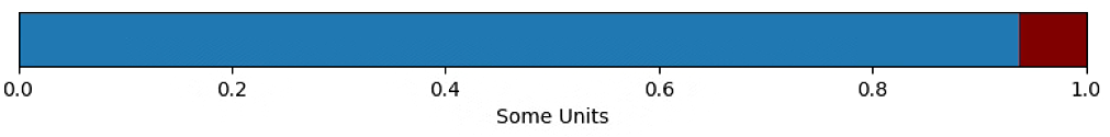
fig, ax = plt.subplots(figsize=(16, 1))
fig.subplots_adjust(bottom=0.5)
fig.colorbar(plt.cm.ScalarMappable(cmap=cmap, norm=norm),boundaries=bounds, ticks=bounds,
cax=ax, orientation='horizontal', label='Some Units')
plt.show()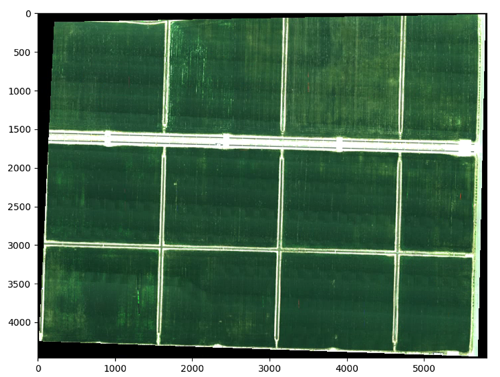
# The color of the circle depends on the NDVI

plt.figure(1)
plt.figure(figsize=(16, 16))
plt.imshow(im_multi_seg.RGB().raster)
ax = plt.gca()

for i, (x1, y1) in enumerate(centers_circles[:2000,:]):
    circle = patches.Circle((x1, y1), r_circle,
                            linewidth=2,
                             edgecolor= cmap(NDVI_circle_index[i]),
                             alpha=0.5,
                             fill = True)
    ax.add_patch(circle)


fig, ax = plt.subplots(figsize=(16, 1))
fig.subplots_adjust(bottom=0.5)

fig.colorbar(plt.cm.ScalarMappable(cmap=cmap, norm=norm),boundaries=bounds, ticks=bounds,
             cax=ax, orientation='horizontal', label='Some Units')
plt.show()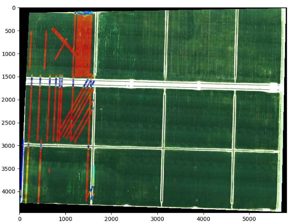
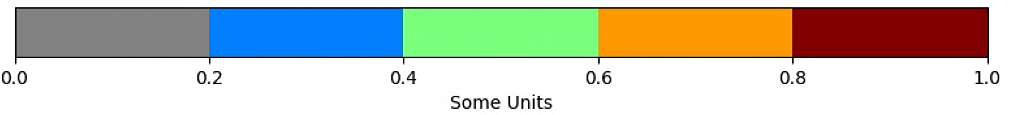
# The color of the circle depends on the OSAVI

r_circle = 10
NDVI = im_multi_seg.OSAVI().raster
NDVI_circle_index = []

for c in centers_circles:

    rr, cc = draw.disk((c[1], c[0]), radius=r_circle, shape=NDVI.shape)
    NDVI_circle_index.append(np.mean(NDVI[rr, cc]))

NDVI_circle_index = np.array(NDVI_circle_index)


n_color = 5
# create the new map
cmap = plt.cm.jet  # define the colormap
# extract all colors from the .jet map
cmaplist = [cmap(i) for i in range(cmap.N)]
# force the first color entry to be grey
cmaplist[0] = (.5, .5, .5, 1.0)

cmap = mpl.colors.LinearSegmentedColormap.from_list('Custom cmap', cmaplist, cmap.N)
# define the bins and normalize
bounds = np.linspace(0, 1, n_color + 1)
norm = mpl.colors.BoundaryNorm(bounds, cmap.N)


NDVI_circle_index[np.isnan(NDVI_circle_index)] = 0
inds = np.digitize(NDVI_circle_index, bounds ,right=False)
NDVI_circle_index_new = [bounds[i-1] for i in inds]


plt.figure(0)
plt.figure(figsize=(16, 16))
plt.imshow(im_multi_seg.RGB().raster)

ax = plt.gca()

plt.figure(1)
plt.figure(figsize=(16, 16))
plt.imshow(im_multi_seg.RGB().raster)
ax = plt.gca()

for i, (x1, y1) in enumerate(centers_circles[:,:]):
    circle = patches.Circle((x1, y1), r_circle,
                            linewidth=2,
                             edgecolor= cmap(NDVI_circle_index_new[i]),
                             alpha=0.5,
                             fill = True)
    ax.add_patch(circle)


fig, ax = plt.subplots(figsize=(16, 1))
fig.subplots_adjust(bottom=0.5)

fig.colorbar(plt.cm.ScalarMappable(cmap=cmap, norm=norm),boundaries=bounds, ticks=bounds,
             cax=ax, orientation='horizontal', label='Some Units')
plt.show()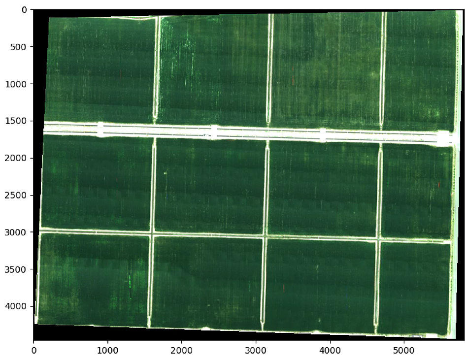
# The color of the circle depends on the OSAVI

plt.hist(NDVI_circle_index)
plt.show()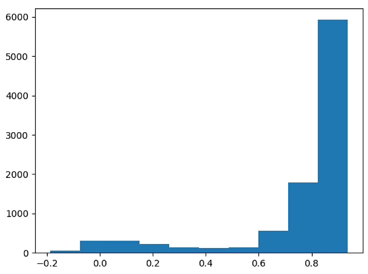
Line Detector.py
# 导包
import numpy as np
from skimage import io
from veg_index import Image_Multi
import matplotlib.pyplot as plt
from matplotlib import path
import matplotlib.patches as patches
import georasters as gr
from scipy import misc
import math
import scipy.ndimage.filters as filters
import scipy.ndimage as ndimage
import Utils
import cv2
from scipy.signal import argrelextrema
from scipy.stats import gaussian_kde
from scipy import ndimage
# 读图
im_red_path = "Barrack A/result_Red.tif"
im_green_path = "Barrack A//result_Green.tif"
im_blue_path = "Barrack A/result_Blue.tif"
im_nir_path = "Barrack A/result_NIR.tif"
im_rededge_path = "Barrack A/result_RedEdge.tif"
im_multi = Image_Multi(im_red_path, im_green_path, im_blue_path, im_nir_path, im_rededge_path)
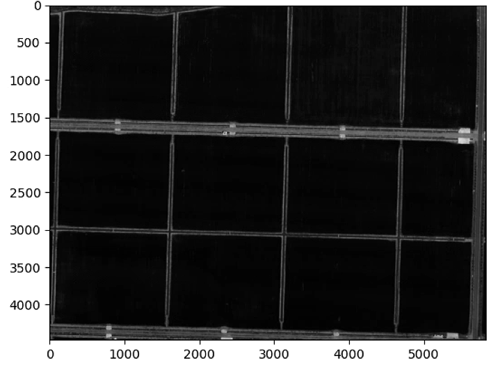
# 分割
List_P = [(1600, 500),(4900, 3600), (1100, 1900), (5900, 1700)]
#List_P = [(500, 3700), (1000, 1900), (4900, 3500), (4000, 5500)]
im_multi_seg = im_multi.Segmentation(List_P)
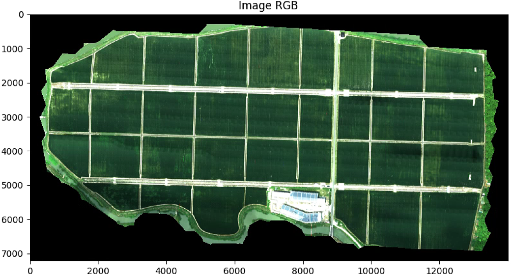
plt.figure(0)
plt.figure(figsize=(10, 10))
plt.imshow(im_multi.RGB().raster)
plt.title( 'Image RGB')
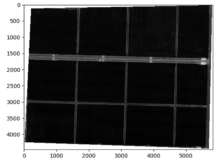
plt.figure(1)
plt.figure(figsize=(10, 10))
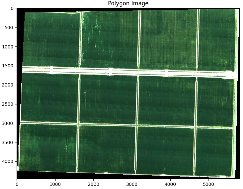
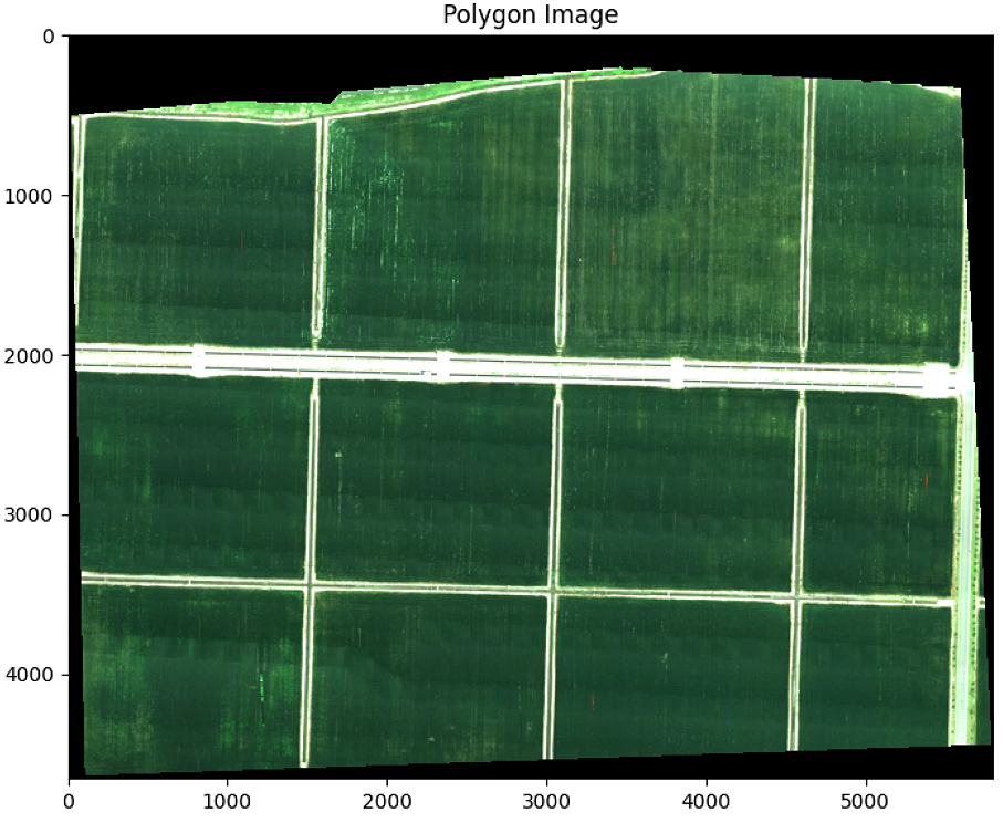
plt.imshow(im_multi_seg.RGB().raster)
plt.title('Polygon Image')
print("Polygon im_multi_seg: " + str(im_multi_seg.list_P))
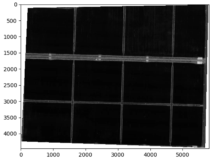
## Subidive image
Points = np.array(im_multi_seg.list_P)
M, maxWidth, maxHeight = Utils.perspectiveTransform(Points)
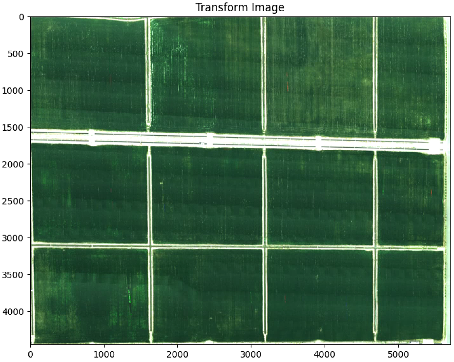
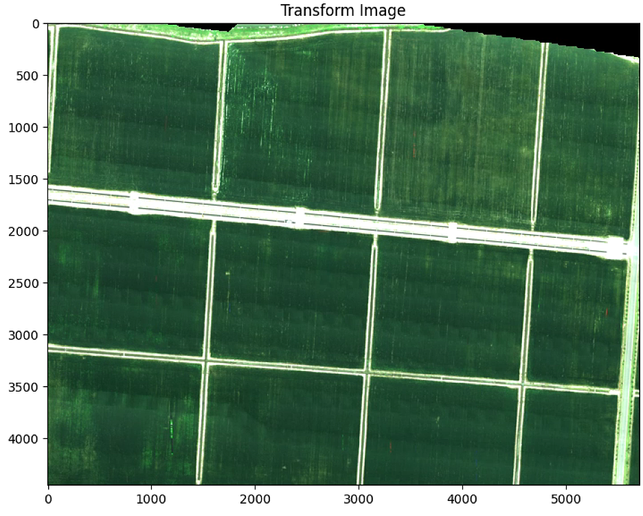
warped = cv2.warpPerspective(im_multi_seg.RGB().raster, M, (maxWidth, maxHeight))
plt.figure(2)
plt.figure(figsize=(10, 10))
plt.imshow(warped)
plt.title('Transform Image')
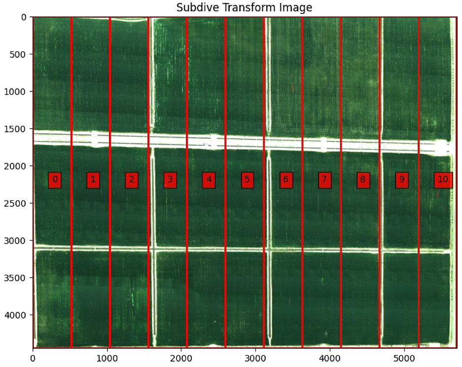
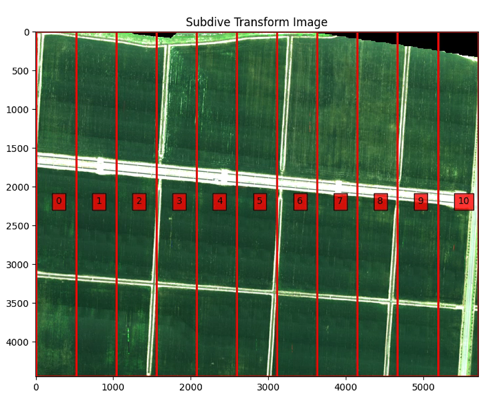
split_Weight, split_Height = 11, 1
sub_division = Utils.subdivision_rect([split_Weight, split_Height], maxWidth, maxHeight)
sub_division_origin = cv2.perspectiveTransform(np.array(sub_division), np.linalg.inv(M))
plt.figure(3)
plt.figure(figsize=(10, 10))
plt.imshow(warped)
plt.title('Subdive Transform Image')
ax = plt.gca()
for i,Poly in enumerate(sub_division):
poly = patches.Polygon(Poly,
linewidth=2,
edgecolor='red',
fill = False)
plt.text(np.mean([x[0] for x in sub_division[i]]), np.mean([y[1] for y in sub_division[i]]) , str(i), bbox=dict(facecolor='red', alpha=0.8))
ax.add_patch(poly)
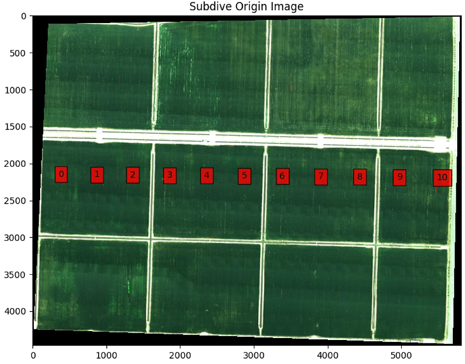
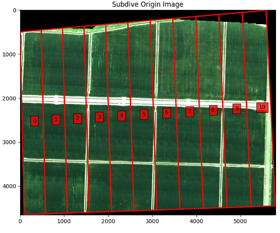
############## Subidive in Origin Image ################
sub_division_origin = cv2.perspectiveTransform(np.array(sub_division), np.linalg.inv(M))
plt.figure(4)
plt.figure(figsize=(10, 10))
plt.imshow(im_multi_seg.RGB().raster)
plt.title('Subdive Origin Image')
ax = plt.gca()
for i,Poly in enumerate(sub_division_origin):
poly = patches.Polygon(Poly,
linewidth=2,
edgecolor='red',
fill = False)
plt.text(np.mean([x[0] for x in sub_division_origin[i]]), np.mean([y[1] for y in sub_division_origin[i]]) , str(i), bbox=dict(facecolor='red', alpha=0.8))
ax.add_patch(poly)
plt.show()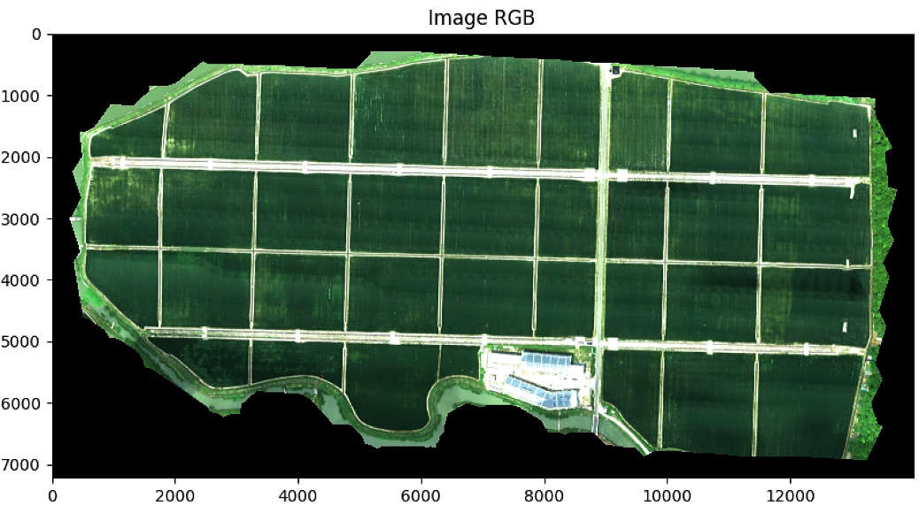
# 子块参数
im_div = im_multi_seg.Segmentation(sub_division_origin[0])
print("Polygon im_div: " + str(im_div.list_P))
#### Transform ####
M, maxWidth, maxHeight = Utils.perspectiveTransform(np.array(im_div.list_P))
NDVI_raster = cv2.warpPerspective(im_div.NDVI().raster, M, (maxWidth, maxHeight))
#NDVI_raster = im_div.NDVI().raster.copy()
NDVI_raster = 2. * (NDVI_raster - np.nanmin(NDVI_raster)) / (np.nanmax(NDVI_raster) - np.nanmin(NDVI_raster))- 1
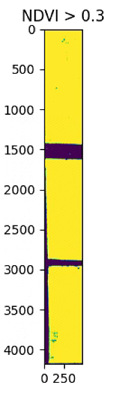
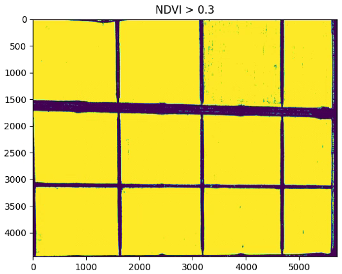
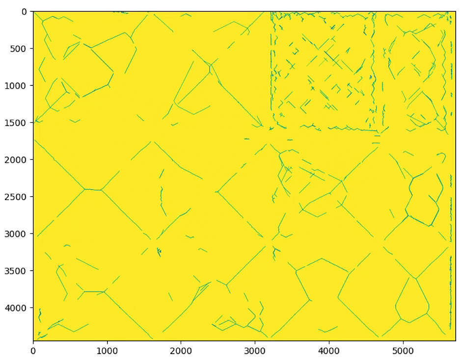
thershold = 0.3
NDVI_raster_th = NDVI_raster > thershold
NDVI_raster_resize = NDVI_raster_th#[2000: 4000, 2000: 4000]
NDVI_raster_bin = np.ones((NDVI_raster_resize.shape))*0
NDVI_raster_bin[NDVI_raster_resize == 1] = 255
plt.figure(0)
plt.imshow(im_div.RGB().raster)
plt.title('Subimage RGB')
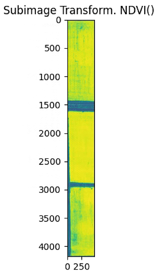
plt.figure(1)
plt.imshow(NDVI_raster)
plt.title('Subimage Transform. NDVI() ')
print(im_div.list_P)
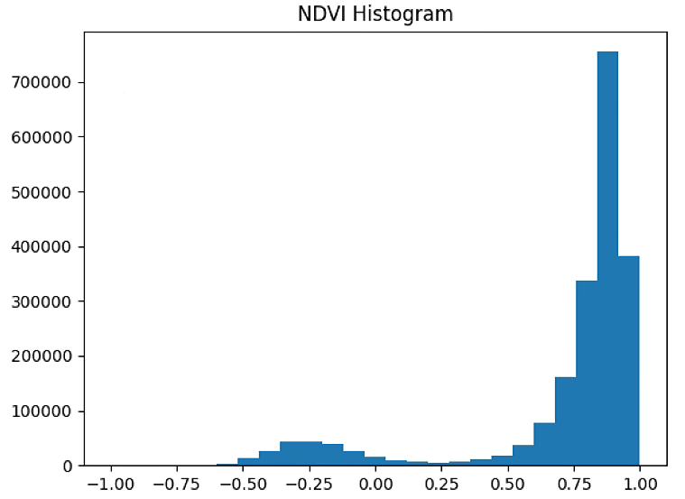
plt.figure(2)
plt.hist(NDVI_raster[~np.isnan(NDVI_raster)], bins = 25)
plt.title('NDVI Histogram')
plt.figure(3)
plt.imshow(NDVI_raster_bin)
plt.title('NDVI > 0.3')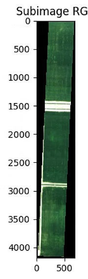
# CANNY Edge

NDVI_raster_bin_copy = NDVI_raster_bin.copy()


low_threshold = 5
high_threshold = 20

kernel_size = 5
blur_gray = cv2.GaussianBlur(NDVI_raster_bin,(kernel_size, kernel_size),2)
edges = cv2.Canny(np.uint8(blur_gray),low_threshold, high_threshold,apertureSize = 3)

height,width = edges.shape
skel = np.zeros([height,width],dtype=np.uint8)      #[height,width,3]
kernel = cv2.getStructuringElement(cv2.MORPH_CROSS, (3,3))
temp_nonzero = np.count_nonzero(edges)

while (np.count_nonzero(edges) != 0 ):
    eroded = cv2.erode(edges,kernel)
    #cv2.imshow("eroded",eroded)
    temp = cv2.dilate(eroded,kernel)
    #cv2.imshow("dilate",temp)
    temp = cv2.subtract(edges,temp)
    skel = cv2.bitwise_or(skel,temp)
    edges = eroded.copy()

plt.figure(2)
plt.figure(figsize=(16, 16))
plt.imshow(skel)
plt.show()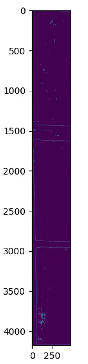
Z1 = np.ones((NDVI_raster_resize.shape))*255
Z2 = np.ones((NDVI_raster_resize.shape))*255
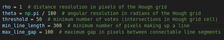
rho = 1 # distance resolution in pixels of the Hough grid
theta = np.pi / 180 # angular resolution in radians of the Hough grid
threshold = 100 # minimum number of votes (intersections in Hough grid cell)
min_line_length = 500 # minimum number of pixels making up a line
max_line_gap = 50 # maximum gap in pixels between connectable line segments
lines = cv2.HoughLines(np.uint8(skel),rho, theta, threshold)
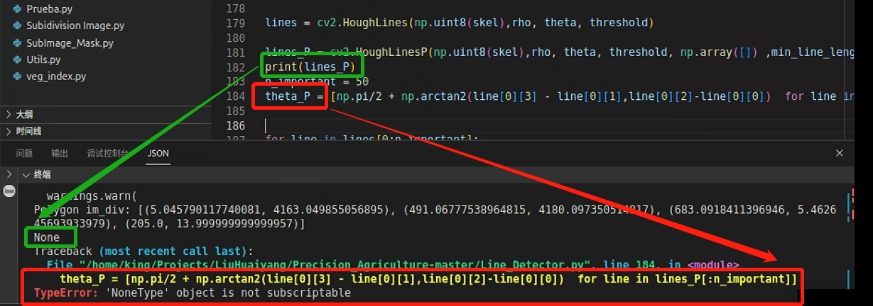
lines_P = cv2.HoughLinesP(np.uint8(skel),rho, theta, threshold, np.array([]) ,min_line_length, max_line_gap)
n_important = 50
theta_P = [np.pi/2 + np.arctan2(line[0][3] - line[0][1],line[0][2]-line[0][0]) for line in lines_P[:n_important]]
for line in lines[0:n_important]:
rho,theta = line[0]
a = np.cos(theta)
b = np.sin(theta)
x0 = a*rho
y0 = b*rho
x1 = int(x0 + 1000*(-b))
y1 = int(y0 + 1000*(a))
x2 = int(x0 - 1000*(-b))
y2 = int(y0 - 1000*(a))
#print((x1,y1,x2,y2))
cv2.line(Z1,(x1,y1),(x2,y2),(0,0,255),2)
for line in lines_P[:n_important]:
x1,y1,x2,y2 = line[0]
cv2.line(Z2,(x1,y1),(x2,y2),(0,0,255),2)
fig, axs = plt.subplots(1, 2, figsize=(16,8))
axs[0].imshow(NDVI_raster_bin)
axs[0].title.set_text('NDVI > 0.3')
axs[1].imshow(skel)
axs[1].title.set_text('Skel_NDVI')
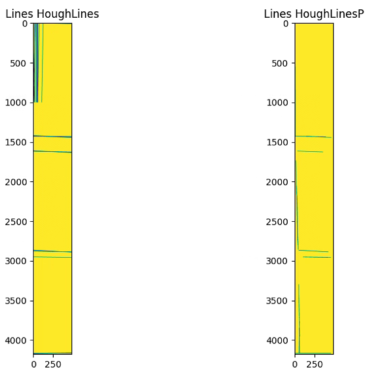
fig, axs = plt.subplots(1, 2, figsize=(16,8))
axs[0].imshow(Z1)
axs[0].title.set_text('Lines HoughLines')
axs[1].imshow(Z2)
axs[1].title.set_text('Lines HoughLinesP')
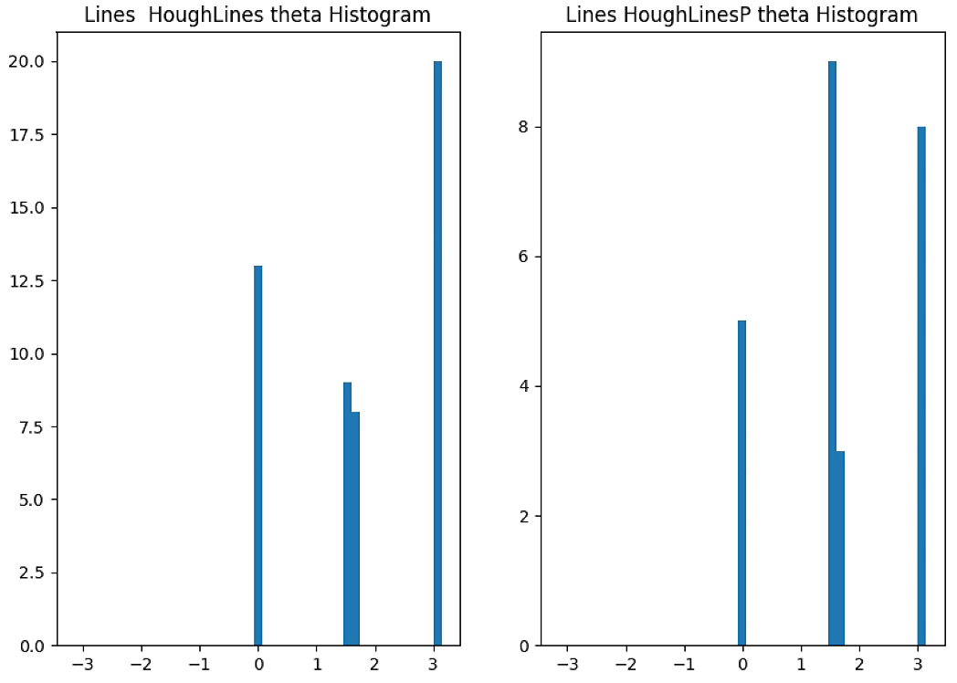
fig, axs = plt.subplots(1, 2, figsize=(16,8))
axs[0].hist(lines[0:n_important,0,1], bins = 45, range=[-np.pi,np.pi])
axs[0].title.set_text('Lines HoughLines theta Histogram')
axs[1].hist(theta_P, bins = 45, range=[-np.pi,np.pi])
axs[1].title.set_text('Lines HoughLinesP theta Histogram')
print(lines.shape)
print(lines_P.shape)
plt.show()这里报了一个错,打印了一下前面的数据类型,发现没检查直线,因此需要调一下参数
调参后

theta = lines[0:n_important,0,1]
h= np.histogram(np.array(theta), bins = 45, range=(-np.pi,np.pi))
peaks = argrelextrema(h[0], np.greater)
h_P = np.histogram(np.array(theta_P), bins = 45, range=(-np.pi,np.pi))
peaks_P = argrelextrema(h_P[0], np.greater)
theta_prop = (h[1][peaks] + h_P[1][peaks_P]) / 2
print(h[1][peaks])
print(h_P[1][peaks_P])
print(theta_prop)
rho = lines[0:50, 0,0]
theta = lines[0:50, 0,1]
xy = np.vstack([theta, rho])
z = gaussian_kde(xy)(xy)
idx = z.argsort()
rho, theta, z = rho[idx], theta[idx], z[idx]
fig, ax = plt.subplots()
ax.scatter(theta, rho, c=z, s=100, edgecolor='')
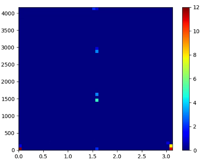
plt.figure(2)
plt.hist2d(theta,rho,(50, 50), cmap=plt.cm.jet)
plt.colorbar() # show color scale
plt.show()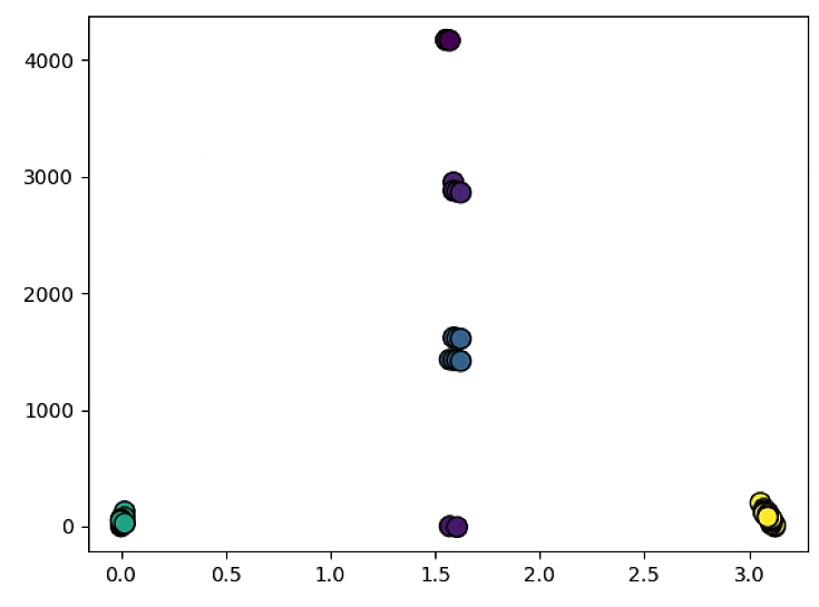
# Analisys total image

#### Transform ####
M, maxWidth, maxHeight = Utils.perspectiveTransform(np.array(im_multi_seg.list_P))
NDVI_raster = cv2.warpPerspective(im_multi_seg.NDVI().raster, M, (maxWidth, maxHeight))
#NDVI_raster = im_div.NDVI().raster.copy()

plt.figure(0)
plt.imshow(NDVI_raster)
plt.title("NDVI Transform")


NDVI_raster = 2. * (NDVI_raster - np.nanmin(NDVI_raster)) / (np.nanmax(NDVI_raster) - np.nanmin(NDVI_raster))- 1
thershold = 0.3
NDVI_raster_th = NDVI_raster > thershold
NDVI_raster_resize = NDVI_raster_th#[2000: 4000, 2000: 4000]
NDVI_raster_bin = np.ones((NDVI_raster_resize.shape))*0
NDVI_raster_bin[NDVI_raster_resize == 1] = 255

plt.figure(1)
plt.hist(NDVI_raster[~np.isnan(NDVI_raster)], bins = 25)
plt.title('NDVI Histogram')

plt.figure(2)
plt.imshow(NDVI_raster_bin)
plt.title('NDVI > 0.3')
plt.show()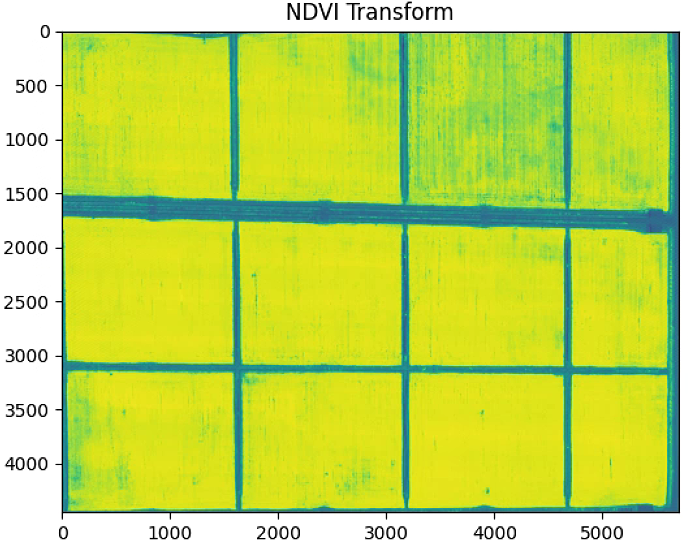
# Edges Lines

kernel_size = 3
edges = cv2.GaussianBlur((NDVI_raster_bin.copy()).astype(np.uint8),(kernel_size, kernel_size),0)
kernel = cv2.getStructuringElement(cv2.MORPH_CROSS,(5, 5))
height,width = edges.shape
skel = np.zeros([height,width],dtype=np.uint8)      #[height,width,3]
temp_nonzero = np.count_nonzero(edges)

while (np.count_nonzero(edges) != 0 ):
    eroded = cv2.erode(edges,kernel)
    #cv2.imshow("eroded",eroded)
    temp = cv2.dilate(eroded,kernel)
    #cv2.imshow("dilate",temp)
    temp = cv2.subtract(edges,temp)
    skel = cv2.bitwise_or(skel,temp)
    edges = eroded.copy()


n_important = 100
"""This function returns the count of labels in a mask image."""
label_im, nb_labels = ndimage.label(skel)#, structure= np.ones((2,2))) ## Label each connect region
label_areas = np.bincount(label_im.ravel())[1:]
keys_max_areas = np.array(sorted(range(len(label_areas)), key=lambda k: label_areas[k], reverse = True)) +1
keys_max_areas = keys_max_areas[:n_important]
L = np.zeros(label_im.shape)
for i in keys_max_areas:
    L[label_im == i] = i

labels = np.unique(L)
label_im = np.searchsorted(labels, L)

plt.figure(0)
plt.figure(figsize=(16, 16))
plt.imshow(skel)
plt.figure(1)
plt.figure(figsize=(16, 16))
plt.imshow(label_im == 0)
plt.show()
其中的n_important = 100的时候

n_important = 300的时候
# Hough Line
Z1 = np.ones((NDVI_raster_resize.shape))*255
Z2 = np.ones((NDVI_raster_resize.shape))*255
skel_filter = label_im>0
rho = 1 # distance resolution in pixels of the Hough grid
theta = np.pi / 180 # angular resolution in radians of the Hough grid
threshold = 100 # minimum number of votes (intersections in Hough grid cell)
min_line_length = 500 # minimum number of pixels making up a line
max_line_gap = 50 # maximum gap in pixels between connectable line segments
lines = cv2.HoughLines(np.uint8(skel_filter),rho, theta, threshold)
lines_P = cv2.HoughLinesP(np.uint8(skel_filter),rho, theta, threshold, np.array([]) ,min_line_length, max_line_gap)
n_important = 100
theta_P = [np.pi/2 + np.arctan2(line[0][3] - line[0][1],line[0][2]-line[0][0]) for line in lines_P[:n_important]]
for line in lines[0:n_important]:
rho,theta = line[0]
a = np.cos(theta)
b = np.sin(theta)
x0 = a*rho
y0 = b*rho
x1 = int(x0 + 1000*(-b))
y1 = int(y0 + 1000*(a))
x2 = int(x0 - 1000*(-b))
y2 = int(y0 - 1000*(a))
#print((x1,y1,x2,y2))
cv2.line(Z1,(x1,y1),(x2,y2),(0,0,255),2)
for line in lines_P[:n_important]:
x1,y1,x2,y2 = line[0]
cv2.line(Z2,(x1,y1),(x2,y2),(0,0,255),2)
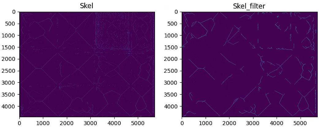
fig, axs = plt.subplots(1, 2, figsize=(16,8))
axs[0].imshow(skel)
axs[0].title.set_text('Skel')
axs[1].imshow(skel_filter)
axs[1].title.set_text('Skel_filter')
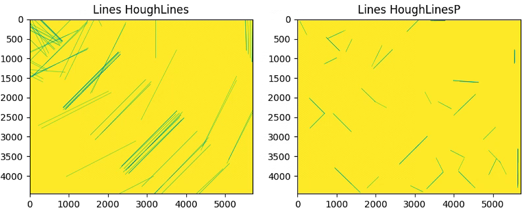
fig, axs = plt.subplots(1, 2, figsize=(16,8))
axs[0].imshow(Z1)
axs[0].title.set_text('Lines HoughLines')
axs[1].imshow(Z2)
axs[1].title.set_text('Lines HoughLinesP')
fig, axs = plt.subplots(1, 2, figsize=(16,8))
axs[0].hist(lines[0:n_important,0,1], bins = 45, range=[-np.pi,np.pi])
axs[0].title.set_text('Lines HoughLines theta Histogram')
axs[1].hist(theta_P, bins = 45, range=[-np.pi,np.pi])
axs[1].title.set_text('Lines HoughLinesP theta Histogram')
print(lines.shape)
print(lines_P.shape)
plt.show()调参

# Search inclinate angle

theta = lines[0:n_important,0,1]

h= np.histogram(np.array(theta), bins = 45, range=(-np.pi,np.pi))
peaks = argrelextrema(h[0], np.greater)

h_P = np.histogram(np.array(theta_P), bins = 45, range=(-np.pi,np.pi))
peaks_P = argrelextrema(h_P[0], np.greater)

theta_prop = (h[1][peaks] + h_P[1][peaks_P]) / 2

# print(h[1][peaks])
# print(h_P[1][peaks_P])
# print(theta_prop)
# Rotate Polygon and subidivide
List_P = [(1600, 500),(4900, 3600), (1100, 1900), (5900, 1700)]
#List_P = [(500, 3700), (1000, 1900), (4900, 3500), (4000, 5500)]
center = (np.mean([point[0] for point in im_multi_seg.list_P]), np.mean([point[1] for point in im_multi_seg.list_P]))
matrix = cv2.getRotationMatrix2D( center=center, angle= -theta_prop[0]*180/np.pi, scale=1)
new_Points = cv2.transform(np.array([List_P]), matrix)[0]
im_multi_seg_new = im_multi.Segmentation(new_Points)
plt.figure(0)
plt.figure(figsize=(10, 10))
plt.imshow(im_multi.RGB().raster)
plt.title( 'Image RGB')
plt.figure(1)
plt.figure(figsize=(10, 10))
plt.imshow(im_multi_seg_new.RGB().raster)
plt.title('Polygon Image')
print("Polygon im_multi_seg: " + str(im_multi_seg_new.list_P))
## Subidive image
Points = np.array(im_multi_seg_new.list_P)
M, maxWidth, maxHeight = Utils.perspectiveTransform(Points)
warped = cv2.warpPerspective(im_multi_seg_new.RGB().raster, M, (maxWidth, maxHeight))
plt.figure(2)
plt.figure(figsize=(10, 10))
plt.imshow(warped)
plt.title('Transform Image')
split_Weight, split_Height = 11, 1
sub_division = Utils.subdivision_rect([split_Weight, split_Height], maxWidth, maxHeight)
sub_division_origin = cv2.perspectiveTransform(np.array(sub_division), np.linalg.inv(M))
plt.figure(3)
plt.figure(figsize=(10, 10))
plt.imshow(warped)
plt.title('Subdive Transform Image')
ax = plt.gca()
for i,Poly in enumerate(sub_division):
poly = patches.Polygon(Poly,
linewidth=2,
edgecolor='red',
fill = False)
plt.text(np.mean([x[0] for x in sub_division[i]]), np.mean([y[1] for y in sub_division[i]]) , str(i), bbox=dict(facecolor='red', alpha=0.8))
ax.add_patch(poly)
############## Subidive in Origin Image ################
sub_division_origin = cv2.perspectiveTransform(np.array(sub_division), np.linalg.inv(M))
plt.figure(4)
plt.figure(figsize=(10, 10))
plt.imshow(im_multi_seg_new.RGB().raster)
plt.title('Subdive Origin Image')
ax = plt.gca()
for i,Poly in enumerate(sub_division_origin):
poly = patches.Polygon(Poly,
linewidth=2,
edgecolor='red',
fill = False)
plt.text(np.mean([x[0] for x in sub_division_origin[i]]), np.mean([y[1] for y in sub_division_origin[i]]) , str(i), bbox=dict(facecolor='red', alpha=0.8))
ax.add_patch(poly)
print([im_multi_seg.list_P])
print(new_Points)
plt.imshow(label_im ==40)
plt.show()这一块可能会报opencv版本的错误,自己根据报错更新一下保本就好
# Rotate Polygon and subidivide

print([im_multi_seg.list_P])
print(new_Points)
plt.imshow(label_im ==40)
Prueba.py
# 导包

import numpy as np
from skimage import io
from veg_index import Image_Multi
import matplotlib.pyplot as plt
from matplotlib import path
from sklearn import cluster
from skimage import data
import cv2
import Utils

import matplotlib.patches as patches
import georasters as gr
from sklearn.metrics import silhouette_score

# 读图

im_red_path = "Barrack A/result_Red.tif"
im_green_path = "Barrack A//result_Green.tif"
im_blue_path = "Barrack A/result_Blue.tif"
im_nir_path = "Barrack A/result_NIR.tif"
im_rededge_path = "Barrack A/result_RedEdge.tif"

im_multi = Image_Multi(im_red_path, im_green_path, im_blue_path, im_nir_path, im_rededge_path)

# 波段显示

plt.figure(figsize=(15, 15))
im_multi.im_red.plot()
plt.title('Red Band')


plt.figure(figsize=(15, 15))
im_multi.im_green.plot()
plt.title('Green Band')


plt.figure(figsize=(15, 15))
im_multi.im_blue.plot()
plt.title('Blue Band')


plt.figure(figsize=(15, 15))
im_multi.im_nir.plot()
plt.title('NIR Band')


plt.figure(figsize=(15, 15))
im_multi.im_rededge.plot()
plt.title('RedEdge Band')
plt.show()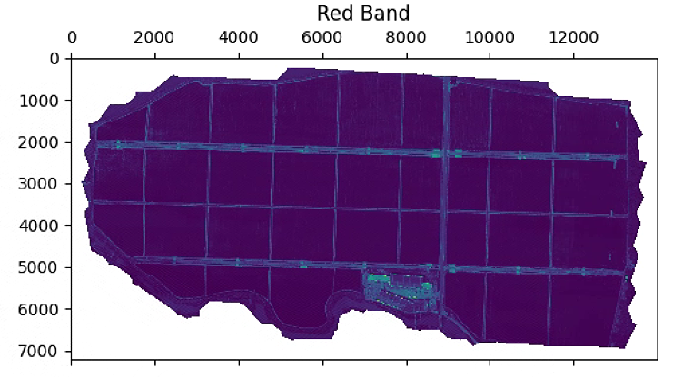
# 植被指数计算

plt.figure(figsize=(15, 15))
im_multi.NDVI().plot()
plt.title('NDVI')

plt.figure(figsize=(15, 15))
im_multi.GNDVI().plot()
plt.title('GNDVI')

plt.figure(figsize=(15, 15))
im_multi.NDRE().plot()
plt.title('NDRE')

plt.figure(figsize=(15, 15))
im_multi.LCI().plot()
plt.title('LCI')

plt.figure(figsize=(15, 15))
im_multi.OSAVI().plot()
plt.title('OSAVI')
plt.show()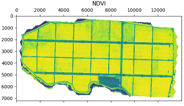
# 植被指数光谱导出

im_multi.NDVI().to_tiff('Barrack A/result_NDVI')
im_multi.GNDVI().to_tiff('Barrack A/result_GNDVI')
im_multi.NDRE().to_tiff('Barrack A/result_NDRE')
im_multi.LCI().to_tiff('Barrack A/result_LCI')
im_multi.OSAVI().to_tiff('Barrack A/result_OSAVI')
# 植被指数直方图显示与保存

n_bins = 8

plt.figure(1)
NDVI_raster = im_multi.NDVI().raster
NDVI_raster = 2. * (NDVI_raster - np.ma.min(NDVI_raster)) / np.ma.ptp(NDVI_raster) - 1
plt.hist(NDVI_raster[~np.isnan(NDVI_raster)], bins = n_bins)
plt.title('NDVI Histogram')
plt.savefig('Barrack A/NDVI_Histogram_'+ str(n_bins))

plt.figure(2)
GNDVI_raster = im_multi.GNDVI().raster
GNDVI_raster = 2. * (GNDVI_raster - np.ma.min(GNDVI_raster)) / np.ma.ptp(GNDVI_raster) - 1
plt.hist(GNDVI_raster[~np.isnan(GNDVI_raster)], bins = n_bins)
plt.title('GNDVI Histogram')
plt.savefig('Barrack A/GNDVI_Histogram_'+ str(n_bins))

plt.figure(3)
NDRE_raster = im_multi.NDRE().raster
NDRE_raster = 2. * (NDRE_raster - np.ma.min(NDRE_raster)) / np.ma.ptp(NDRE_raster) - 1
plt.hist(NDRE_raster[~np.isnan(NDRE_raster)], bins = n_bins)
plt.title('NDRE Histogram')
plt.savefig('Barrack A/NDRE_Histogram_'+ str(n_bins))

plt.figure(4)
LCI_raster = im_multi.LCI().raster
LCI_raster = 2. * (LCI_raster - np.ma.min(LCI_raster)) / np.ma.ptp(LCI_raster) - 1
plt.hist(LCI_raster[~np.isnan(LCI_raster)], bins = n_bins)
plt.title('LCI Histogram')
plt.savefig('Barrack A/LCI_Histogram_'+ str(n_bins))

plt.figure(5)
OSAVI_raster = im_multi.OSAVI().raster
OSAVI_raster = 2. * (OSAVI_raster - np.ma.min(OSAVI_raster)) / np.ma.ptp(OSAVI_raster) - 1
plt.hist(OSAVI_raster[~np.isnan(OSAVI_raster)], bins = n_bins)
plt.title('OSAVI Histogram')
plt.savefig('Barrack A/OSAVI_Histogram_'+ str(n_bins))

plt.figure(6)
OSAVI_raster = im_multi.OSAVI_16().raster
OSAVI_raster = 2. * (OSAVI_raster - np.ma.min(OSAVI_raster)) / np.ma.ptp(OSAVI_raster) - 1
plt.hist(OSAVI_raster[~np.isnan(OSAVI_raster)], bins = n_bins)
plt.title('OSAVI_16 Histogram')
plt.savefig('Barrack A/OSAVI_16_Histogram_'+ str(n_bins))
plt.show()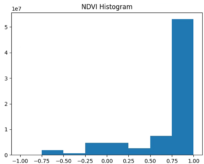
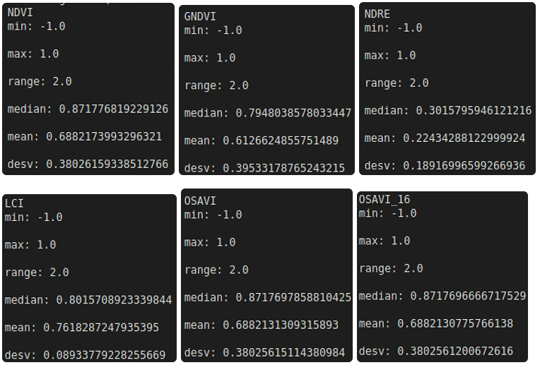
# 植被指数数据分析与输出

L = ["min: ", "max: ", "range: ", "median: ", "mean: ", "desv: "]
name = ["NDVI", "GNDVI", "NDRE", "LCI", "OSAVI", "OSAVI_16"]
func_raster = [im_multi.NDVI, im_multi.GNDVI, im_multi.NDRE, im_multi.LCI, im_multi.OSAVI, im_multi.OSAVI_16]


for name, f in zip(name,func_raster):
    raster = f().raster
    raster = 2. * (raster - np.min(raster)) / np.ptp(raster) - 1
    statistics = [np.ma.min(raster), np.ma.max(raster), np.ma.ptp(raster),
                  np.ma.median(raster), np.ma.mean(raster), np.ma.std(raster)]

    file1 = open("Barrack A/{}_statistics.txt".format(name),"w") # 指定路径输出
    file1.writelines([L[i]+ str(statistics[i]) + "\n" for i in range(len(L))])
    file1.close() #to change file access modes
    print(name)
    for i in [L[i]+ str(statistics[i]) + "\n" for i in range(len(L))]: print(i)
# Segmentation

import matplotlib.patches as patches
import georasters as gr

epsilon = 10
Red=im_multi.im_red
List_P = [(2200,2000), (2000, 4000), (3000, 3400), (3600, 1500)]

(xmin, xsize, x, ymax, y, ysize) = Red.geot
x_rect = min([f[0] for f in List_P]) - epsilon
y_rect = min([f[1] for f in List_P]) - epsilon
h_rect = max([f[1] for f in List_P]) - min([f[1] for f in List_P]) + 2 * epsilon
w_rect = max([f[0] for f in List_P]) - min([f[0] for f in List_P]) + 2 * epsilon

poly = path.Path(List_P)
xv,yv = np.meshgrid(range(Red.raster.shape[1]), range(Red.raster.shape[0]))
flags = ~poly.contains_points(np.hstack((xv.flatten()[:,np.newaxis], yv.flatten()[:,np.newaxis])))
Seg_tot = Red.raster.copy()
Seg_tot[flags.reshape(Red.raster.shape)] = np.nan

plt.figure()
plt.imshow(Red.raster, cmap = 'gray')


ax = plt.gca()

rect = patches.Rectangle((x_rect, y_rect),
                 w_rect,
                 h_rect,
                 linewidth=2,
                 edgecolor='cyan',
                 fill = False)

ax.add_patch(rect)
poly = patches.Polygon(List_P,
                 linewidth=2,
                 edgecolor='red',
                 fill = False)


ax.add_patch(poly)


plt.figure()
plt.imshow(Seg_tot, cmap = 'gray')


### Re parametrice

new_Red = gr.GeoRaster(Red.raster[y_rect: y_rect + h_rect, x_rect : x_rect + w_rect],
                     (xmin + xsize * w_rect, xsize, x, ymax + ysize * h_rect, y, ysize),
                     nodata_value=Red.nodata_value,
                     projection=Red.projection,
                     datatype=Red.datatype)

List_P = [(x - x_rect, y - y_rect) for x,y in List_P]
poly = path.Path(List_P)
xv,yv = np.meshgrid(range(w_rect), range(h_rect))
flags = ~poly.contains_points(np.hstack((xv.flatten()[:,np.newaxis], yv.flatten()[:,np.newaxis])))


Seg_crop = new_Red.raster.copy()
Seg_crop[flags.reshape(new_Red.raster.shape)] = np.nan

plt.figure()
plt.imshow(new_Red.raster, cmap = 'gray')


plt.figure()
plt.imshow(Seg_crop, cmap = 'gray')
plt.show()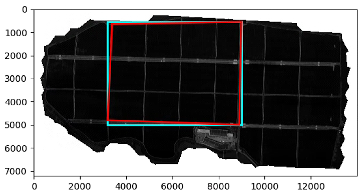

# Segmentation with veg-index function

List_P = [(2200,2000), (2000, 4000), (3000, 3400), (3600, 1500)]

im_multi_seg = im_multi.Segmentation(List_P)

epsilon = 0
x_rect = min([f[0] for f in List_P]) - epsilon
y_rect = min([f[1] for f in List_P]) - epsilon
h_rect = max([f[1] for f in List_P]) - min([f[1] for f in List_P]) + 2 * epsilon
w_rect = max([f[0] for f in List_P]) - min([f[0] for f in List_P]) + 2 * epsilon

plt.figure()
plt.imshow(im_multi.im_red.raster, cmap = 'gray')


ax = plt.gca()

rect = patches.Rectangle((x_rect, y_rect),
                 w_rect,
                 h_rect,
                 linewidth=2,
                 edgecolor='cyan',
                 fill = False)
ax.add_patch(rect)
poly = patches.Polygon(List_P,
                 linewidth=2,
                 edgecolor='red',
                 fill = False)


ax.add_patch(poly)


plt.figure()
plt.imshow(im_multi_seg.im_red.raster, cmap = 'gray')

plt.figure()
plt.imshow(im_multi_seg.OSAVI().raster, cmap = 'gray')
plt.show()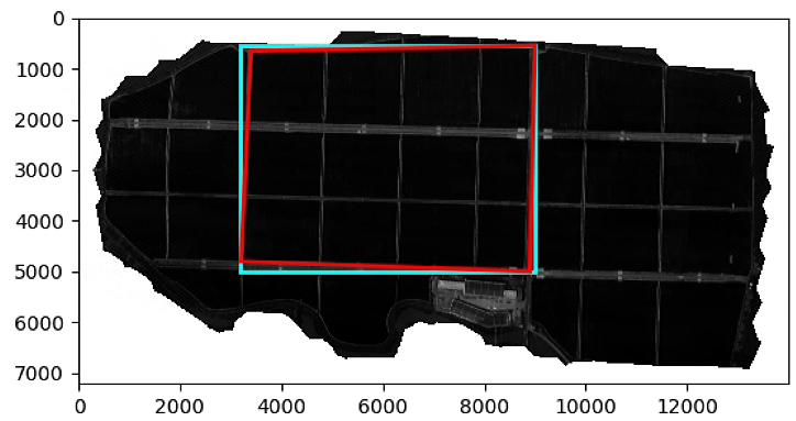
# RGB and Kmean
def rgb2gray(rgb):
return np.dot(rgb[...,:3], [0.2989, 0.5870, 0.1140])
def km_clust(array, n_clusters):
# Create a line array, the lazy way
if len(array.shape) == 3:
X = array.reshape((-1, array.shape[-1]))
else :
X = array.reshape((-1, 1))
# Define the k-means clustering problem
k_m = cluster.KMeans(n_clusters = n_clusters, n_init=4)
# Solve the k-means clustering problem
k_m.fit(X)
# Get the coordinates of the clusters centres as a 1D array
values = k_m.cluster_centers_.squeeze()
# Get the label of each point
labels = k_m.labels_
return(values, labels, k_m)
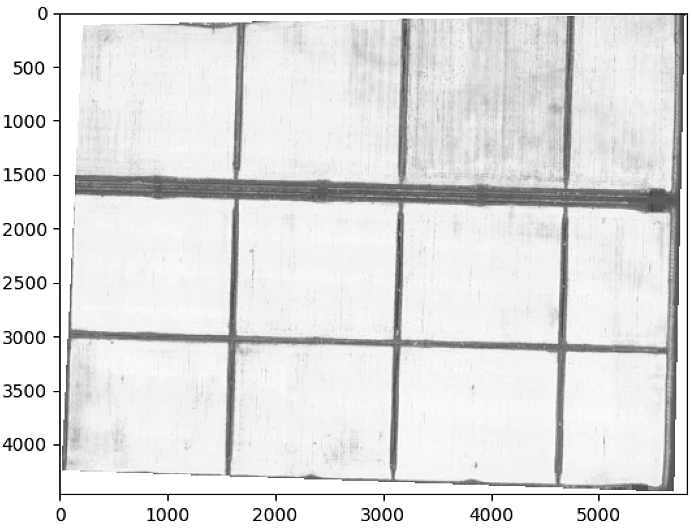
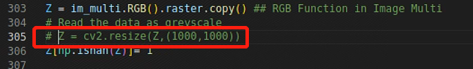
Z = im_multi.RGB().raster.copy() ## RGB Function in Image Multi
# Read the data as greyscale
Z = cv2.resize(Z,(1000,1000))
Z[np.isnan(Z)]= 1
Z = cv2.GaussianBlur(Z,(5, 5), 2)
plt.figure(0)
plt.imshow(Z)
img = Z#[:,:,1]
# Group similar grey levels using 8 clusters
values, labels, km = km_clust(img, n_clusters = 4)
print (values.shape)
print (labels.shape)
# Create the segmented array from labels and values
img_segm = np.array([values[label] for label in labels]) #np.choose(labels, values)
# Reshape the array as the original image
img_segm.shape = img.shape
# Get the values of min and max intensity in the original image
vmin = img.min()
vmax = img.max()
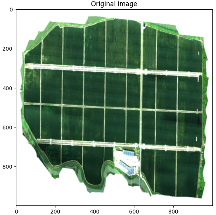
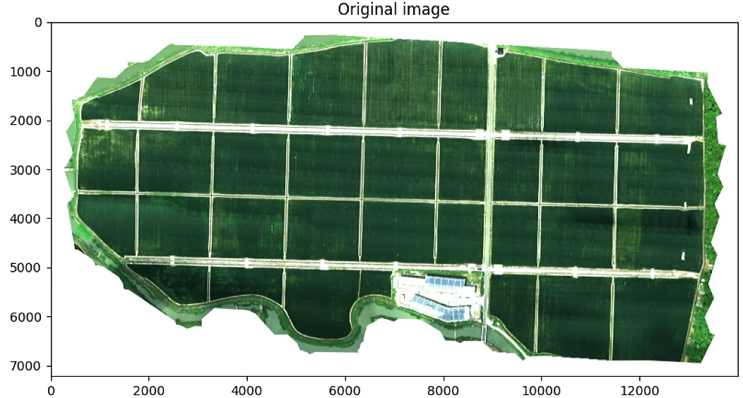
# Plot the original image
plt.figure(figsize = (16,16))
plt.imshow(Z, cmap = 'jet', vmin=vmin, vmax=vmax)
plt.title('Original image')
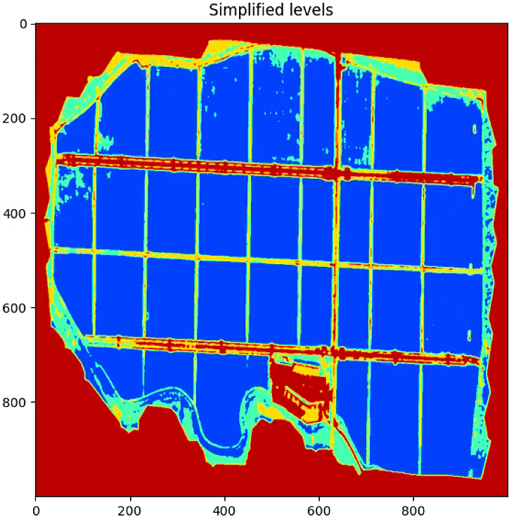
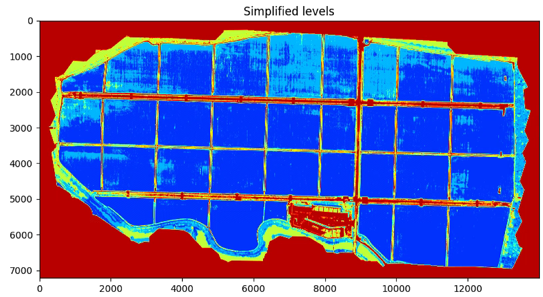
# Plot the simplified color image
if len(img_segm.shape) == 3:
gray = rgb2gray(img_segm)
else: gray = img_segm
plt.figure(figsize = (16,16))
plt.imshow(gray, cmap = 'jet', vmin=vmin, vmax=vmax)
plt.title('Simplified levels')
plt.show()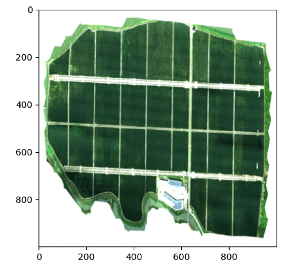
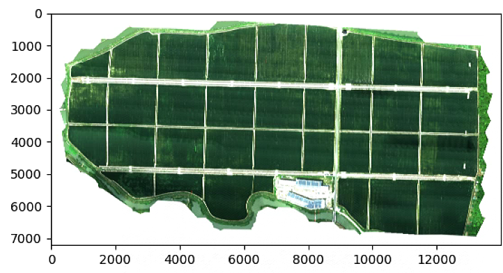
由于源码中加了resize,所以比例看着怪怪的,这里注释掉resize
可以看出注释掉resize比例正常了,但是计算速度下降非常大
# Search K
n_max = 11
img = cv2.resize(img,(200,200))
sil = []
distortions = []
X = img.reshape((-1, 3))
for i in range(2,n_max):
#print(i)
values, labels, k_m = km_clust(img, n_clusters = i)
distortions.append(k_m.inertia_)
sil.append(silhouette_score(X[::5,:], labels[::5], metric = 'euclidean'))
plt.figure()
plt.plot(range(2, n_max), distortions, marker='o')
plt.xlabel('Number of clusters')
plt.ylabel('Distortion')
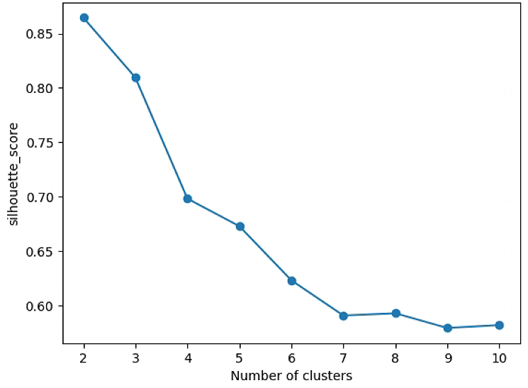
plt.figure()
plt.plot(range(2, n_max), sil, marker='o')
plt.xlabel('Number of clusters')
plt.ylabel('silhouette_score')
plt.show()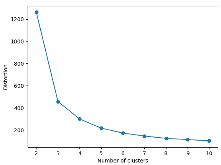
# K-means with coordinate

List_P = [(2200,2000), (2000, 4000), (3000, 3400), (3600, 1500)]

im_multi_seg = im_multi.Segmentation(List_P)

Z = im_multi_seg.RGB().raster.copy() ## RGB Function in Image Multi
#Z = im_multi_seg.NDVI().raster.copy()
#Z[Z>4000] = 4000
#Z = Z/ (np.nanmax(Z) - np.nanmin(Z))

Z = cv2.resize(Z,(1000, 1000))

Z = cv2.GaussianBlur(Z,(5, 5), 1)
Z[np.isnan(Z)]= np.nanmax(Z)

img_segm = Utils.kmeans_image(Z, n_clusters = 3)

# Plot the simplified color image
if len(img_segm.shape) == 3:
    gray = Utils.rgb2gray(img_segm)
else: gray = img_segm


vmin = Z.min()
vmax = Z.max()

plt.figure(figsize = (16,16))
plt.imshow(Z, cmap = 'gray')

plt.figure(figsize = (16,16))
plt.imshow(gray, cmap = 'ocean', vmin=vmin, vmax=vmax)
plt.title('Simplified levels without spatial coordinate')

Subidivision_Mask.py
# 导包

import numpy as np
from skimage import io
from veg_index import Image_Multi
import matplotlib.pyplot as plt
from matplotlib import path
import matplotlib.patches as patches
import georasters as gr

from scipy import misc
import math
import scipy.ndimage.filters as filters
import scipy.ndimage as ndimage
import Utils
import cv2

import time

im_red_path = "Barrack A/result_Red.tif"
im_green_path = "Barrack A//result_Green.tif"
im_blue_path = "Barrack A/result_Blue.tif"
im_nir_path = "Barrack A/result_NIR.tif"
im_rededge_path = "Barrack A/result_RedEdge.tif"

im_multi = Image_Multi(im_red_path, im_green_path, im_blue_path, im_nir_path, im_rededge_path)

List_P = [(1600, 500),(4800, 3600), (1100, 1900), (5500, 1900)]
#List_P = [(500, 3700), (1000, 1900), (4900, 3600), (4000, 5500)]

im_multi_seg = im_multi.Segmentation(List_P)

Points = np.array(im_multi_seg.list_P)
Points_order = Utils.order_points_rect(Points)

M, maxWidth, maxHeight = Utils.perspectiveTransform(Points)

plt.figure(0)
plt.figure(figsize=(16, 16))
plt.imshow(im_multi.RGB().raster)

plt.figure(1)
plt.figure(figsize=(16, 16))
plt.imshow(im_multi_seg.RGB().raster)
print(im_multi_seg.list_P)
plt.show()
# Divide lmage and rotate subimage
# top-left, top-right, bottom-right, and bottom-left
split_Weight, split_Height = 15, 3
sub_division = Utils.subdivision_rect([split_Weight, split_Height], maxWidth, maxHeight, 0.01)

sub_division_origin = cv2.perspectiveTransform(np.array(sub_division), np.linalg.inv(M))
print(len(sub_division))

List_P = np.uint(sub_division_origin)
List_new_P = []

for P in List_P:
    #P = List_P[3]
    im = im_multi_seg.Segmentation(P)
    NDVI = im.NDVI().raster

    #NDVI = 2. * (NDVI - np.nanmin(NDVI)) / (np.nanmax(NDVI) - np.nanmin(NDVI))- 1
    #blur[np.isnan(blur)] = 0
    Points = np.array(im.list_P)

    M, maxWidth, maxHeight = Utils.perspectiveTransform(Utils.order_points_rect(Points))

    warped = cv2.warpPerspective(NDVI, M, (maxWidth, maxHeight))
    warped[np.isnan(warped)] = 0

    # Otsu
    blur = cv2.GaussianBlur(warped * 255,(5,5),0).astype('uint8')
    ret3,th3 = cv2.threshold(blur,0,255,cv2.THRESH_BINARY+cv2.THRESH_OTSU)

    n_important = 100
    skel_filter = Utils.skeleton(th3, n_important = 100)

    theta_prop = Utils.angle_lines(skel_filter,  n_important = 100, angle_resolution = 720,
                                   threshold = 100, min_line_length = 200,
                                   max_line_gap = 50, plot = False)


    #center = (im.list_P[0][0], im.list_P[0][1])
    #center_pol = center
    center = (np.mean([point[0] for point in P]), np.mean([point[1] for point in P]))
    matrix = cv2.getRotationMatrix2D(center=center, angle= -theta_prop*180/np.pi, scale=1)


    new_P = cv2.transform(np.array([P]), matrix)[0]

    #im_multi_seg_new = im_multi_seg.Segmentation(new_P)

    #new_Points = np.array(im_multi_seg_new.list_P)
    List_new_P.append(new_P)
    #print(theta_prop)

plt.figure(0)
plt.imshow(im_multi_seg.RGB().raster.copy())
plt.title('Subdive Origin Image')
ax = plt.gca()

for i,Poly in enumerate(List_P):
    poly = patches.Polygon(Poly,
                     linewidth=2,
                     edgecolor='red',
                     fill = False)
    plt.text(np.mean([x[0]  for x in Poly]), np.mean([y[1]  for y in Poly]) , str(i),  bbox=dict(facecolor='red', alpha=0.8))

    ax.add_patch(poly)


plt.figure(1)
plt.imshow(im_multi_seg.RGB().raster.copy())
plt.title('Subdive Origin Image')
ax = plt.gca()

ax.scatter(center[0], center[1], marker='o', color='g', label='point')
for i,Poly in enumerate(List_new_P):

    poly = patches.Polygon(Poly,
                     linewidth=2,
                     edgecolor='red',
                     fill = False)
    plt.text(np.mean([x[0]  for x in Poly]), np.mean([y[1]  for y in Poly]) , str(i),  bbox=dict(facecolor='red', alpha=0.8))

    ax.add_patch(poly)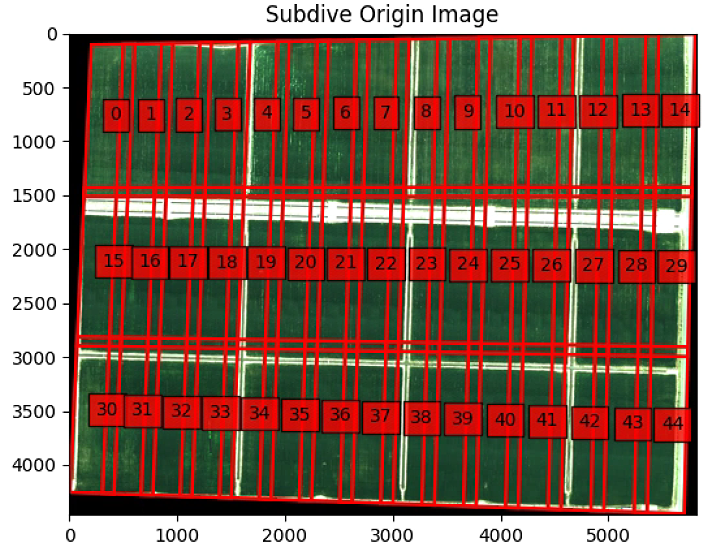

# 颜色变换
P = List_new_P[13]
P = Utils.order_points_rect(P)
im = im_multi_seg.Segmentation(P)

Points = np.array(im.list_P)
M_sub, maxWidth, maxHeight = Utils.perspectiveTransform(Utils.order_points_rect(Points))
RGB = cv2.warpPerspective(im.RGB().raster, M_sub, (maxWidth, maxHeight))

RGB = cv2.GaussianBlur(RGB,(21,21),0).astype('float32')
HSV = Utils.rgb2hsv(RGB)

H = HSV[:, :, 0]
H2 = H.copy()
#H2 = cv2.GaussianBlur(H2,(9,9),0).astype('float32')
H2[H > 210] = 0
H2[H < 210] = 1
H2[H < 70] = 0
H2 = H2.astype('uint8')

### Change Green color to NDVI
NDVI = cv2.warpPerspective(im.NDVI().raster, M_sub, (maxWidth, maxHeight))
H2 = (NDVI > 0.6).astype('uint8')


plt.figure(0, figsize = (14,14))
plt.imshow(RGB)
plt.title('Subdive Origin Image')


plt.figure(1, figsize = (14,14))
plt.imshow(H2)
plt.title('HSV')


plt.figure(3, figsize = (14,14))
plt.imshow(im.NDVI().raster > 0.3)
plt.title('NDVI > 0.3')

plt.figure(4, figsize = (14,14))
plt.imshow(im.NDVI().raster > 0.6)
plt.title('NDVI > 0.6')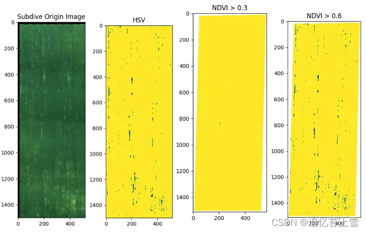
### Create kernel rotate #########333
size_kernel = 10
kernel = np.ones((size_kernel, 5) , np.uint8)  # note this is a vertical kernel
#kernel = np.ones((5, 5) , np.uint8)

erode = cv2.erode(H2,kernel)
closing = cv2.morphologyEx(erode, cv2.MORPH_CLOSE, kernel)
skel = Utils.skeleton(closing, n_important = -1)


closing_skel = cv2.morphologyEx(skel.astype(float), cv2.MORPH_CLOSE, kernel)
closing_skel = cv2.morphologyEx(closing_skel, cv2.MORPH_CLOSE, kernel)

label_im, nb_labels = ndimage.label(closing_skel)#, structure= np.ones((2,2))) ## Label each connect region
label_areas = np.bincount(label_im.ravel())[1:]

th = 20 #np.mean(label_areas) # Th

L = np.zeros(label_im.shape)

for i in range(nb_labels):
    if label_areas[i] > th:
        L[label_im == (i + 1) ] = 1

L = cv2.morphologyEx(L, cv2.MORPH_CLOSE, kernel)

plt.figure(0, figsize = (14,14))
plt.imshow(H2)
plt.title('segmentate')

plt.figure(1, figsize = (14,14))
plt.imshow(closing)
plt.title('closing')

plt.figure(1, figsize = (14,14))
plt.imshow(skel)
plt.title('skel')

plt.figure(2, figsize = (14,14))
plt.imshow(closing_skel)
plt.title('closing_skel')

plt.figure(3, figsize = (14,14))
plt.imshow(L)
plt.title('L')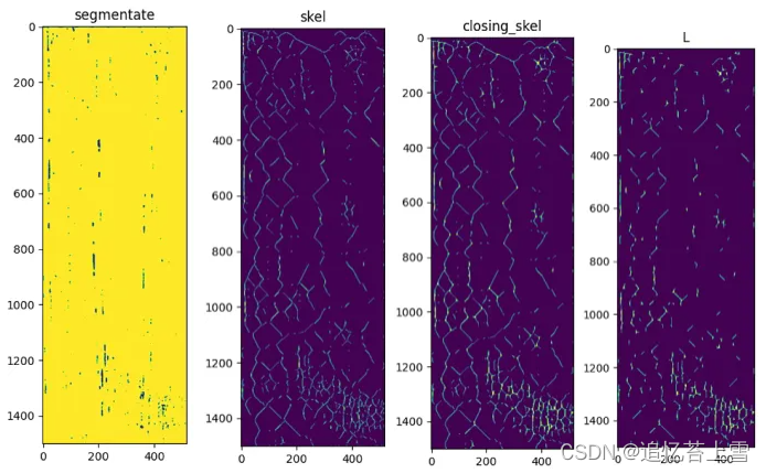
label_im, nb_labels = ndimage.label(L)#, structure= np.ones((2,2))) ## Label each connect region
label_areas = np.bincount(label_im.ravel())[1:]

List_Centroid_WH = []
for i in range(nb_labels):

    I = np.zeros(label_im.shape)
    I[label_im == (i + 1)] = 1
    # calculate moments of binary image
    Moments = cv2.moments(I)
    # calculate x,y coordinate of center
    cX = int(Moments["m10"] / Moments["m00"])
    cY = int(Moments["m01"] / Moments["m00"])
    cnts, hierarchy = cv2.findContours(I.astype('uint8'), cv2.RETR_EXTERNAL,cv2.CHAIN_APPROX_SIMPLE)
    width = np.max([x[0][0] for x in cnts[0]]) - np.min([x[0][0] for x in cnts[0]])
    height = np.max([y[0][1] for y in cnts[0]]) - np.min([y[0][1] for y in cnts[0]])
    List_Centroid_WH.append((cX, cY, width, height))

x_min = np.min([x[0] - x[2]/2 for x in List_Centroid_WH])
x_max = np.max([x[0] + x[2]/2 for x in List_Centroid_WH])
y_min = np.min([y[1] - y[3]/2 for y in List_Centroid_WH])
y_max = np.max([y[1] + y[3]/2 for y in List_Centroid_WH])

L_xw = sorted([[x[0],x[2]] for x in List_Centroid_WH])

## Filter width separation
th = np.mean(L_xw, axis=0)[1]
L_filter = [L_xw[0][0]]
L_width = [L_xw[0][1]]
for i in range(len(L_xw)):
    if (abs(L_filter[-1] - L_xw[i][0]) > th):
        L_filter.append(L_xw[i][0])
        L_width.append(L_xw[i][1])

#filter mean dif separation
dif = [L_filter[i] - L_filter[i-1] for i in range(1, len(L_filter))]
th = np.mean(dif).astype('int') + np.std(dif).astype('int') - 10
L_filter_2 = [L_filter[0]]
L_width_2 = [L_width[0]]
for i in range(len(L_filter)):
    if (abs(L_filter_2[-1] - L_filter[i]) > th):
        L_filter_2.append(L_filter[i])
        L_width_2.append(L_width[i])

####################### lista de poligonos ################
List_lines = [] #(top-left, top-right,bottom-right, bottom-left
avg_width = 1 #np.mean(L_width_2)/3#L_width[i]
for i in range(len(L_filter_2)):


    top_left = (int(L_filter_2[i] - avg_width/2) , y_min)
    top_right = (int(L_filter_2[i] + avg_width/2) , y_min)
    bottom_right = (int(L_filter_2[i] + avg_width/2) , y_max)
    bottom_left = (int(L_filter_2[i] - avg_width/2) , y_max)
    if  int(L_filter_2[i] - avg_width/2) > L.shape[1]:
        print('Salio')
        break

    List_lines.append((top_left, top_right, bottom_right, bottom_left))

List_lines_origin = cv2.perspectiveTransform(np.array(List_lines), np.linalg.inv(M_sub)) # In subdivide image
List_lines_origin_complete = List_lines_origin - Utils.order_points_rect(Points)[0] + Utils.order_points_rect(P)[0] # In image complet # Put line in big image

plt.figure(0, figsize = (16,16))
plt.imshow(RGB)
plt.title('Subdive Origin Image')
ax = plt.gca()

for i,Poly in enumerate(List_lines):
    poly = patches.Polygon(Poly,
                     linewidth=2,
                     edgecolor='red',
                     alpha=0.5,
                     fill = True)
    plt.text(np.mean([x[0]  for x in Poly]), np.mean([y[1]  for y in Poly]) , str(i),  bbox=dict(facecolor='red', alpha=0.8))

    ax.add_patch(poly)

plt.figure(1, figsize = (16,16))
plt.imshow(im.RGB().raster)
plt.title('Subdive Origin Image')
ax = plt.gca()

for i,Poly in enumerate(List_lines_origin):
    poly = patches.Polygon(Poly,
                     linewidth=2,
                     edgecolor='red',
                     alpha=0.5,
                     fill = True)
    plt.text(np.mean([x[0]  for x in Poly]), np.mean([y[1]  for y in Poly]) , str(i),  bbox=dict(facecolor='red', alpha=0.8))

    ax.add_patch(poly)

plt.figure(2)
plt.figure(figsize=(16, 16))
plt.imshow(im_multi_seg.RGB().raster)

ax = plt.gca()


for i,Poly in enumerate(List_lines_origin_complete):
    poly = patches.Polygon(Poly,
                     linewidth=2,
                     edgecolor='red',
                     alpha=0.5,
                     fill = True)
    plt.text(np.mean([x[0]  for x in Poly]), np.mean([y[1]  for y in Poly]) , str(i),  bbox=dict(facecolor='red', alpha=0.8))

    ax.add_patch(poly)
plt.show()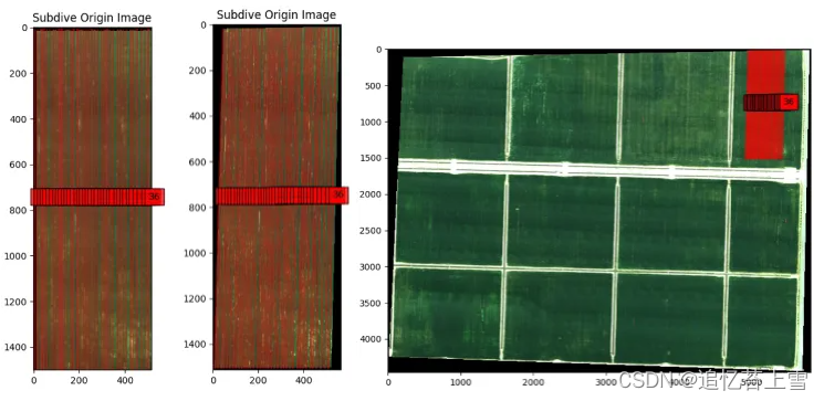
plt.figure(0, figsize = (16,16))
plt.imshow(im.RGB().raster)
plt.title('Subdive Origin Image')
ax = plt.gca()

r_circle = 10
for i,Poly in enumerate(List_lines_origin):
    poly = patches.Polygon(Poly,
                         linewidth=2,
                         edgecolor='red',
                         alpha=0.5,
                         fill = True)
    plt.text(np.mean([x[0]  for x in Poly]), np.mean([y[1]  for y in Poly]) , str(i),  bbox=dict(facecolor='red', alpha=0.8))

    ax.add_patch(poly)

    P1 = np.mean(Poly[0:2], axis=0)
    P2 = np.mean(Poly[2:4], axis=0)

    distance = np.linalg.norm(P1-P2)
    n_step = int(distance/(r_circle *2))
    centers = np.array([P1 * t/n_step + P2 * (n_step-t)/n_step for t in range(n_step + 1)])

    for x1, y1 in centers:
        circle = patches.Circle((x1, y1), r_circle,
                                linewidth=2,
                                 edgecolor='blue',
                                 alpha=0.5,
                                 fill = True)
        ax.add_patch(circle)
plt.show()
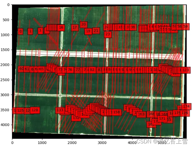
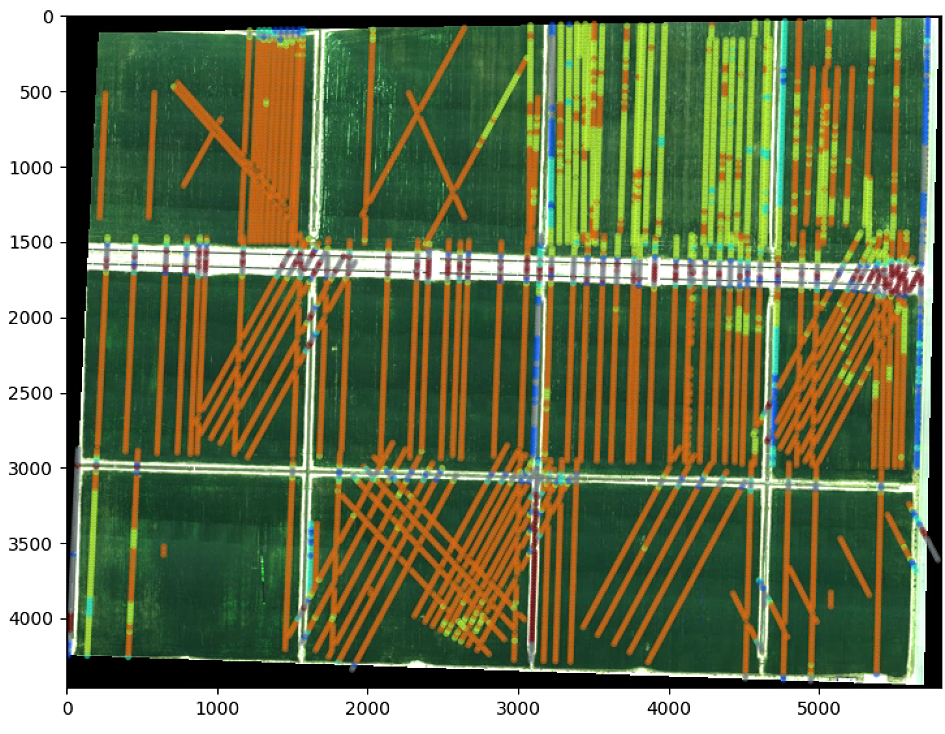
# All lines GREEN

List_lines_origin_complete =  np.ones((0,4,2))

gaussian_kernel_size = 21
th_green_up = 210
th_green_down = 70
vertical_kernel_size_h = 10
vertical_kernel_size_w = 5
th_small_areas = 30
lines_width = 1
merge_bt_line = 10

for P in List_new_P:

    P = Utils.order_points_rect(P)
    im = im_multi_seg.Segmentation(P)

    Points = np.array(im.list_P)
    M_sub, maxWidth, maxHeight = Utils.perspectiveTransform(Utils.order_points_rect(Points))
    RGB = cv2.warpPerspective(im.RGB().raster, M_sub, (maxWidth, maxHeight))

    RGB = cv2.GaussianBlur(RGB,(gaussian_kernel_size, gaussian_kernel_size),0).astype('float32')
    HSV = Utils.rgb2hsv(RGB)

    H = HSV[:, :, 0]
    H2 = H.copy()
    #H2 = cv2.GaussianBlur(H2,(9,9),0).astype('float32')
    H2[H > th_green_up] = 0
    H2[H < th_green_up] = 1
    H2[H < th_green_down] = 0
    H2 = H2.astype('uint8')

    ### Create kernel rotate #########333

    kernel = np.ones((vertical_kernel_size_h, vertical_kernel_size_w) , np.uint8)  # note this is a vertical kernel
    #kernel = np.ones((5, 5) , np.uint8)

    erode = cv2.erode(H2,kernel)
    closing = cv2.morphologyEx(erode, cv2.MORPH_CLOSE, kernel)
    skel = Utils.skeleton(closing, n_important = -1)


    closing_skel = cv2.morphologyEx(skel.astype(float), cv2.MORPH_CLOSE, kernel)
    closing_skel = cv2.morphologyEx(closing_skel, cv2.MORPH_CLOSE, kernel)

    label_im, nb_labels = ndimage.label(closing_skel)#, structure= np.ones((2,2))) ## Label each connect region
    label_areas = np.bincount(label_im.ravel())[1:]


    L = np.zeros(label_im.shape)

    for i in range(nb_labels):
        if label_areas[i] > th_small_areas:
            L[label_im == (i + 1) ] = 1

    L = cv2.morphologyEx(L, cv2.MORPH_CLOSE, kernel)

    label_im, nb_labels = ndimage.label(L)#, structure= np.ones((2,2))) ## Label each connect region
    label_areas = np.bincount(label_im.ravel())[1:]

    List_Centroid_WH = []
    for i in range(nb_labels):

        I = np.zeros(label_im.shape)
        I[label_im == (i + 1)] = 1
        # calculate moments of binary image
        Moments = cv2.moments(I)
        # calculate x,y coordinate of center
        cX = int(Moments["m10"] / Moments["m00"])
        cY = int(Moments["m01"] / Moments["m00"])
        cnts, hierarchy = cv2.findContours(I.astype('uint8'), cv2.RETR_EXTERNAL,cv2.CHAIN_APPROX_SIMPLE)
        width = np.max([x[0][0] for x in cnts[0]]) - np.min([x[0][0] for x in cnts[0]])
        height = np.max([y[0][1] for y in cnts[0]]) - np.min([y[0][1] for y in cnts[0]])
        List_Centroid_WH.append((cX, cY, width, height))

    x_min = np.min([x[0] - x[2]/2 for x in List_Centroid_WH])
    x_max = np.max([x[0] + x[2]/2 for x in List_Centroid_WH])
    y_min = np.min([y[1] - y[3]/2 for y in List_Centroid_WH])
    y_max = np.max([y[1] + y[3]/2 for y in List_Centroid_WH])

    L_xw = sorted([[x[0],x[2]] for x in List_Centroid_WH])

    ## Filter width separation
    th = np.mean(L_xw, axis=0)[1]
    L_filter = [L_xw[0][0]]
    L_width = [L_xw[0][1]]
    for i in range(len(L_xw)):
        if (abs(L_filter[-1] - L_xw[i][0]) > th):
            L_filter.append(L_xw[i][0])
            L_width.append(L_xw[i][1])

    #filter mean dif separation
    dif = [L_filter[i] - L_filter[i-1] for i in range(1, len(L_filter))]
    th = np.mean(dif).astype('int') + np.std(dif).astype('int') - merge_bt_line
    L_filter_2 = [L_filter[0]]
    L_width_2 = [L_width[0]]
    for i in range(len(L_filter)):
        if (abs(L_filter_2[-1] - L_filter[i]) > th):
            L_filter_2.append(L_filter[i])
            L_width_2.append(L_width[i])

    ####################### lista de poligonos ################
    List_lines = [] #(top-left, top-right,bottom-right, bottom-left
    avg_width = lines_width #np.mean(L_width_2)/3#L_width[i]
    for i in range(len(L_filter_2)):


        top_left = (int(L_filter_2[i] - avg_width/2) , y_min)
        top_right = (int(L_filter_2[i] + avg_width/2) , y_min)
        bottom_right = (int(L_filter_2[i] + avg_width/2) , y_max)
        bottom_left = (int(L_filter_2[i] - avg_width/2) , y_max)
        if  int(L_filter_2[i] - avg_width/2) > L.shape[1]:
            break

        List_lines.append((top_left, top_right, bottom_right, bottom_left))

    List_lines_origin = cv2.perspectiveTransform(np.array(List_lines), np.linalg.inv(M_sub)) # In subdivide image
    List_lines_origin_complete = np.concatenate((List_lines_origin_complete,
                                                    List_lines_origin - Utils.order_points_rect(Points)[0] + Utils.order_points_rect(P)[0]))# In image complet # Put line in big image


plt.figure(2)
plt.figure(figsize=(16, 16))
plt.imshow(im_multi_seg.RGB().raster)

ax = plt.gca()


for i,Poly in enumerate(List_lines_origin_complete):
    poly = patches.Polygon(Poly,
                     linewidth=2,
                     edgecolor='red',
                     alpha=0.5,
                     fill = True)
    plt.text(np.mean([x[0]  for x in Poly]), np.mean([y[1]  for y in Poly]) , str(i),  bbox=dict(facecolor='red', alpha=0.8))

    ax.add_patch(poly)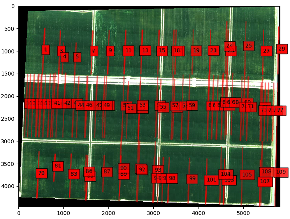
# All Image NDVI
List_lines_origin_complete =  np.ones((0, 4, 2))

th_NDVI = 0.6
vertical_kernel_size_h = 10
vertical_kernel_size_w = 5
th_small_areas = 30
lines_width = 1
merge_bt_line = 10

for P in List_new_P:

    P = Utils.order_points_rect(P)
    im = im_multi_seg.Segmentation(P)

    Points = np.array(im.list_P)
    M_sub, maxWidth, maxHeight = Utils.perspectiveTransform(Utils.order_points_rect(Points))

    NDVI = cv2.warpPerspective(im.NDVI().raster, M_sub, (maxWidth, maxHeight))
    H2 = (NDVI > th_NDVI).astype('uint8')
    ### Create kernel rotate #########333

    kernel = np.ones((vertical_kernel_size_h, vertical_kernel_size_w) , np.uint8)  # note this is a vertical kernel
    #kernel = np.ones((5, 5) , np.uint8)

    erode = cv2.erode(H2,kernel)
    closing = cv2.morphologyEx(erode, cv2.MORPH_CLOSE, kernel)
    skel = Utils.skeleton(closing, n_important = -1)


    closing_skel = cv2.morphologyEx(skel.astype(float), cv2.MORPH_CLOSE, kernel)
    closing_skel = cv2.morphologyEx(closing_skel, cv2.MORPH_CLOSE, kernel)

    label_im, nb_labels = ndimage.label(closing_skel)#, structure= np.ones((2,2))) ## Label each connect region
    label_areas = np.bincount(label_im.ravel())[1:]


    L = np.zeros(label_im.shape)

    for i in range(nb_labels):
        if label_areas[i] > th_small_areas:
            L[label_im == (i + 1) ] = 1

    L = cv2.morphologyEx(L, cv2.MORPH_CLOSE, kernel)

    label_im, nb_labels = ndimage.label(L)#, structure= np.ones((2,2))) ## Label each connect region
    label_areas = np.bincount(label_im.ravel())[1:]

    List_Centroid_WH = []
    for i in range(nb_labels):

        I = np.zeros(label_im.shape)
        I[label_im == (i + 1)] = 1
        # calculate moments of binary image
        Moments = cv2.moments(I)
        # calculate x,y coordinate of center
        cX = int(Moments["m10"] / Moments["m00"])
        cY = int(Moments["m01"] / Moments["m00"])
        cnts, hierarchy = cv2.findContours(I.astype('uint8'), cv2.RETR_EXTERNAL,cv2.CHAIN_APPROX_SIMPLE)
        width = np.max([x[0][0] for x in cnts[0]]) - np.min([x[0][0] for x in cnts[0]])
        height = np.max([y[0][1] for y in cnts[0]]) - np.min([y[0][1] for y in cnts[0]])
        List_Centroid_WH.append((cX, cY, width, height))

    x_min = np.min([x[0] - x[2]/2 for x in List_Centroid_WH])
    x_max = np.max([x[0] + x[2]/2 for x in List_Centroid_WH])
    y_min = np.min([y[1] - y[3]/2 for y in List_Centroid_WH])
    y_max = np.max([y[1] + y[3]/2 for y in List_Centroid_WH])

    L_xw = sorted([[x[0],x[2]] for x in List_Centroid_WH])

    ## Filter width separation
    th = np.mean(L_xw, axis=0)[1]
    L_filter = [L_xw[0][0]]
    L_width = [L_xw[0][1]]
    for i in range(len(L_xw)):
        if (abs(L_filter[-1] - L_xw[i][0]) > th):
            L_filter.append(L_xw[i][0])
            L_width.append(L_xw[i][1])

    #filter mean dif separation
    dif = [L_filter[i] - L_filter[i-1] for i in range(1, len(L_filter))]
    th = np.mean(dif).astype('int') + np.std(dif).astype('int') - merge_bt_line
    L_filter_2 = [L_filter[0]]
    L_width_2 = [L_width[0]]
    for i in range(len(L_filter)):
        if (abs(L_filter_2[-1] - L_filter[i]) > th):
            L_filter_2.append(L_filter[i])
            L_width_2.append(L_width[i])

    ####################### lista de poligonos ################
    List_lines = [] #(top-left, top-right,bottom-right, bottom-left
    avg_width = lines_width #np.mean(L_width_2)/3#L_width[i]
    for i in range(len(L_filter_2)):


        top_left = (int(L_filter_2[i] - avg_width/2) , y_min)
        top_right = (int(L_filter_2[i] + avg_width/2) , y_min)
        bottom_right = (int(L_filter_2[i] + avg_width/2) , y_max)
        bottom_left = (int(L_filter_2[i] - avg_width/2) , y_max)
        if  int(L_filter_2[i] - avg_width/2) > L.shape[1]:
            break

        List_lines.append((top_left, top_right, bottom_right, bottom_left))

    List_lines_origin = cv2.perspectiveTransform(np.array(List_lines), np.linalg.inv(M_sub)) # In subdivide image
    List_lines_origin_complete = np.concatenate((List_lines_origin_complete,
                                                List_lines_origin - Utils.order_points_rect(Points)[0] + Utils.order_points_rect(P)[0]))# In image complet # Put line in big image


plt.figure(0)
plt.figure(figsize=(16, 16))
plt.imshow(im_multi_seg.RGB().raster)

ax = plt.gca()


for i,Poly in enumerate(List_lines_origin_complete):
    poly = patches.Polygon(Poly,
                     linewidth=2,
                     edgecolor='red',
                     alpha=0.5,
                     fill = True)
    plt.text(np.mean([x[0]  for x in Poly]), np.mean([y[1]  for y in Poly]) , str(i),  bbox=dict(facecolor='red', alpha=0.8))

    ax.add_patch(poly)
plt.show()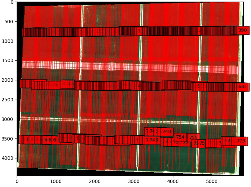
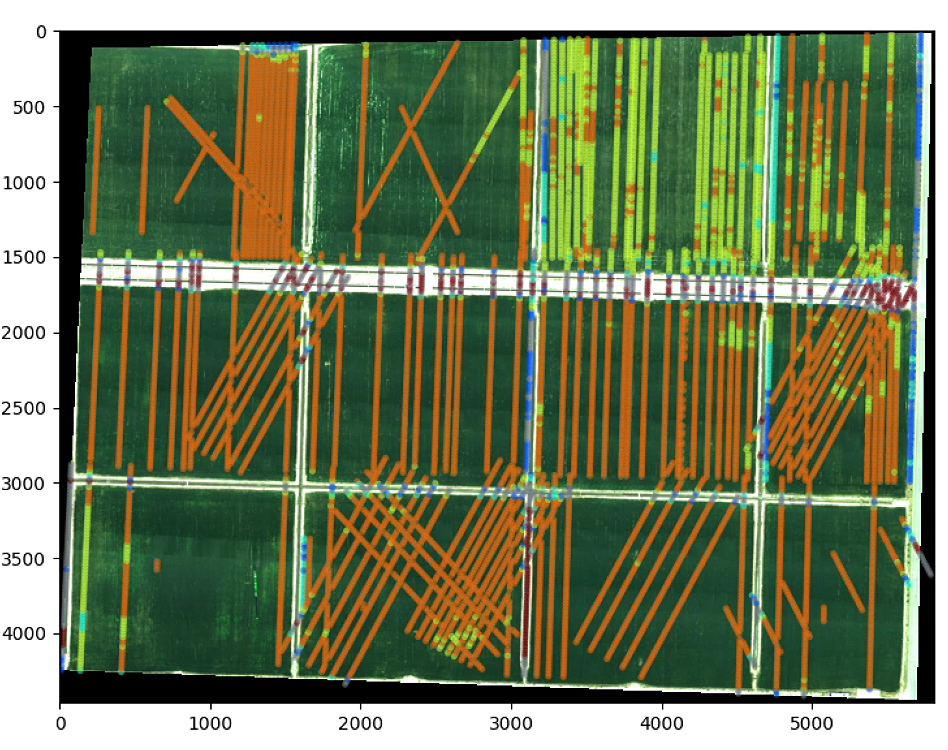
centers_filter = np.ones((0, 2))
centers = np.ones((0, 2))
r_circle = 10

for i,Poly in enumerate(List_lines_origin_complete[:n_important]):

    P1 = np.mean(Poly[0:2], axis=0)
    P2 = np.mean(Poly[2:4], axis=0)

    distance = np.linalg.norm(P1-P2)
    n_step = int(distance/(r_circle *2 + 1))

    centers = np.concatenate((centers, np.array([P1 * t/n_step + P2 * (n_step-t)/n_step for t in range(n_step + 1)]).astype(int)))

centers = (np.unique(np.uint(centers), axis = 0)).astype(np.float)

start = time.time()
    ### Filter circle so close
centers_filter = np.concatenate((centers_filter, np.array([centers[0]])))

for c in centers[1:]:
    if np.min(np.linalg.norm(c - centers_filter, axis=1)) > 2 * r_circle:

        centers_filter = np.concatenate((centers_filter,np.array([c])))

centers_filter = np.array(centers_filter)

end = time.time()
print(end - start)
plt.figure(0)
plt.figure(figsize=(16, 16))
plt.imshow(im_multi_seg.RGB().raster)

ax = plt.gca()

for i,Poly in enumerate(List_lines_origin_complete[:20,:,:]):
    poly = patches.Polygon(Poly,
                     linewidth=2,
                     edgecolor='red',
                     alpha=0.5,
                     fill = True)
    plt.text(np.mean([x[0]  for x in Poly]), np.mean([y[1]  for y in Poly]) , str(i),  bbox=dict(facecolor='red', alpha=0.8))

    ax.add_patch(poly)

for x1, y1 in centers_filter[:1000,:]:
    circle = patches.Circle((x1, y1), r_circle,
                            linewidth=2,
                             edgecolor='blue',
                             alpha=0.5,
                             fill = True)
    ax.add_patch(circle)
plt.show()
print(centers_filter.shape)
print(centers.shape)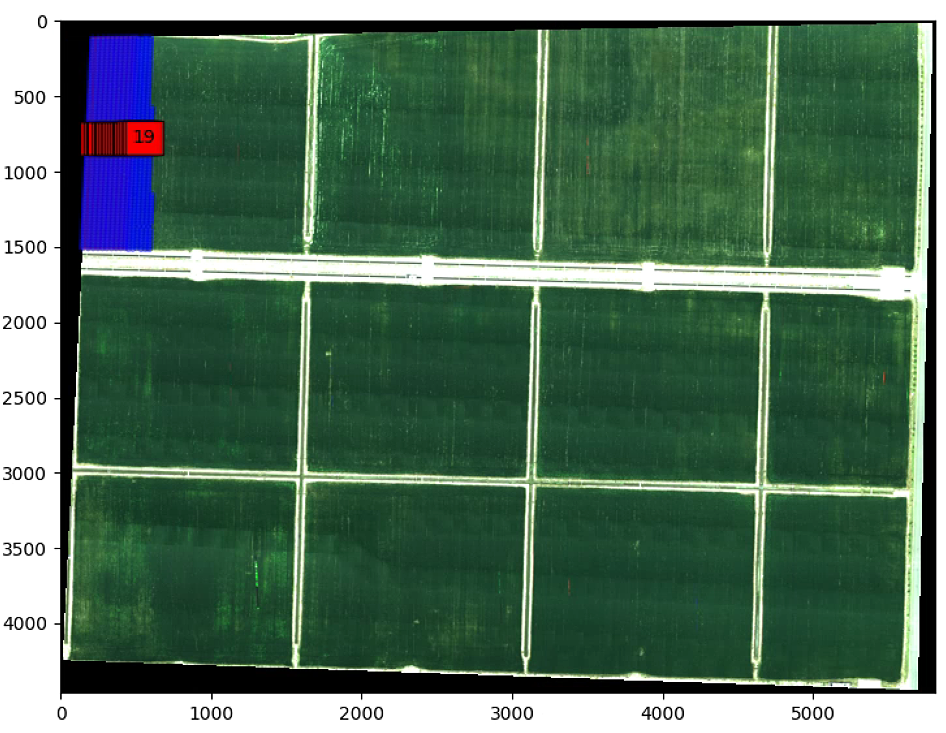


 1万+
1万+


 被折叠的 条评论
为什么被折叠?
被折叠的 条评论
为什么被折叠?
 到【灌水乐园】发言


