T-SNE图

最近实习让画一个图，一个图神经网络的工作，给的其他论文中的样例是这样的：

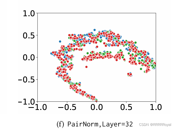
拿到这个样例真的很懵逼，首先不知道横纵坐标是什么意思，各种颜色是什么意思。研究了半天感觉不同颜色应该是代表着监督学习中的不同的类别，这个图的作用应该是看数据的分布，但是还是不知道横纵坐标是什么意思。
后来查了半天才知道这玩意叫T-SNE图，一种广泛用于高维数据可视化的降维算法。通过将高维数据嵌入到二维或三维空间中，使得对复杂的数据结构的理解更加直观。
全称叫t-Distributed Stochastic Neighbor Embedding, t-分布随机邻域嵌入
本质就是把多维数据转化到二维进行可视化，最后用python完成了绘图：

from __future__ import division, print_function
import random
import argparse
import torch
import torch.optim as optim
from torch.autograd import Variable
from gra import get_center_1
from dataprocess import *
from models import GAT, SpGAT
from am_utils import load_data, load_graph
from config import Config
from sklearn.manifold import TSNE

seed = 42
random.seed(seed)
np.random.seed(seed)
torch.manual_seed(seed)
torch.cuda.manual_seed(seed)
dataname = 'acm'

# Load data and initialize model
config_file = "am/60" + dataname + ".ini"
config = Config(config_file)
labelrate = 60
sadj, fadj = load_graph(labelrate, config)
features, labels, idx_train1, idx_test = load_data(config)
adj = sadj
tail_adj = adj
adj = torch.FloatTensor(adj.todense())

idx_train = idx_train1[:1050]
idx_val = idx_train1[1050:]
hidden = 8
nb_heads = 8
dropout = 0.6
alpha = 0.2
lr = 0.01
weight_decay = 5e-4
model = GAT(nfeat=features.shape[1],
            nhid=hidden,
            nclass=int(labels.max()) + 1,
            dropout=dropout,
            nheads=nb_heads,
            alpha=alpha)
optimizer = optim.Adam(model.parameters(),
                       lr=lr,
                       weight_decay=weight_decay)

model.cuda()
features = features.cuda()
adj = adj.cuda()
labels = labels.cuda()
idx_train = idx_train.cuda()
idx_val = idx_val.cuda()
idx_test = idx_test.cuda()

clusters = 7
k=0.1
# gai
shape = adj.shape
cal_node = (shape[0] / clusters) * 0.05
m = np.ceil(cal_node).astype(int)
ori_fe_num = features.shape[0]
features, adj = get_center_1(features, clusters, adj,k, m)
features, adj, labels = Variable(features), Variable(adj), Variable(labels)

best_epoch='pklfile/model4acmlr=0.0001.pkl'

# Restore best model
print('Loading'+best_epoch+'epoch')


model.load_state_dict(torch.load(best_epoch))

features, adj = get_center_1(features, clusters, adj,k, m)
features, adj, labels = Variable(features), Variable(adj), Variable(labels)

print(features.shape)
print(adj.shape)
print(labels.shape)

# t-SNE visualization
encoded_features = model(features, adj)

# Convert embeddings to numpy
encoded_features_np = encoded_features.detach().cpu().numpy()

# t-SNE
tsne = TSNE(n_components=2, random_state=0)
tsne_results = tsne.fit_transform(encoded_features_np)

def plot_tsne(X, labels):
    import matplotlib.pyplot as plt
    import numpy as np

    print(f'TSNE results shape: {X.shape}')
    print(f'Labels shape: {labels.shape}')

    # 检查 X 和 labels 是否长度一致
    if X.shape[0] != labels.shape[0]:
        raise ValueError("The number of samples in tsne_results and labels_np are not equal.")
    # 坐标归一化，缩放到[-1, 1]
    X_min, X_max = X.min(), X.max()
    X = 2 * (X - X_min) / (X_max - X_min) - 1
    # colors = plt.cm.get_cmap('tab10', len(np.unique(labels)))
    #设置画布底色全部为白色
    # 去除图例
    plt.legend().remove()
    colors = plt.cm.get_cmap('hsv', len(np.unique(labels)))
    for i in np.unique(labels):
        correct_indices = np.where(labels == i)[0]
        plt.scatter(X[correct_indices, 0], X[correct_indices, 1], c=[colors(i)], label=str(i), s=30,edgecolors='w',linewidths=1.0)
    # plt.legend()
    plt.xlim(-1, 1)
    plt.ylim(-1, 1)
    plt.xticks(np.arange(-1, 1.5, 0.5))
    plt.yticks(np.arange(-1, 1.5, 0.5))
    plt.figtext(0.5, 0.01, 'Acm', ha='center', fontsize=12)
    plt.show()


# Visualize
labels_np = labels.cpu().numpy()
print(len(tsne_results))
print(len(labels_np) )
# 过滤掉没有标签的数据
if len(labels_np) < len(tsne_results):
    tsne_results = tsne_results[:len(labels_np)]
elif len(labels_np) > len(tsne_results):
    labels_np = labels_np[:len(tsne_results)]

# 检查长度是否一致
assert tsne_results.shape[0] == labels_np.shape[0], "The number of samples in tsne_results and labels_np are not equal."

plot_tsne(tsne_results, labels_np)
# draw_graph_tsne(tsne_results, adj.cpu().numpy(), labels_np)