梯度下降法代码实践

梯度下降法最简步骤

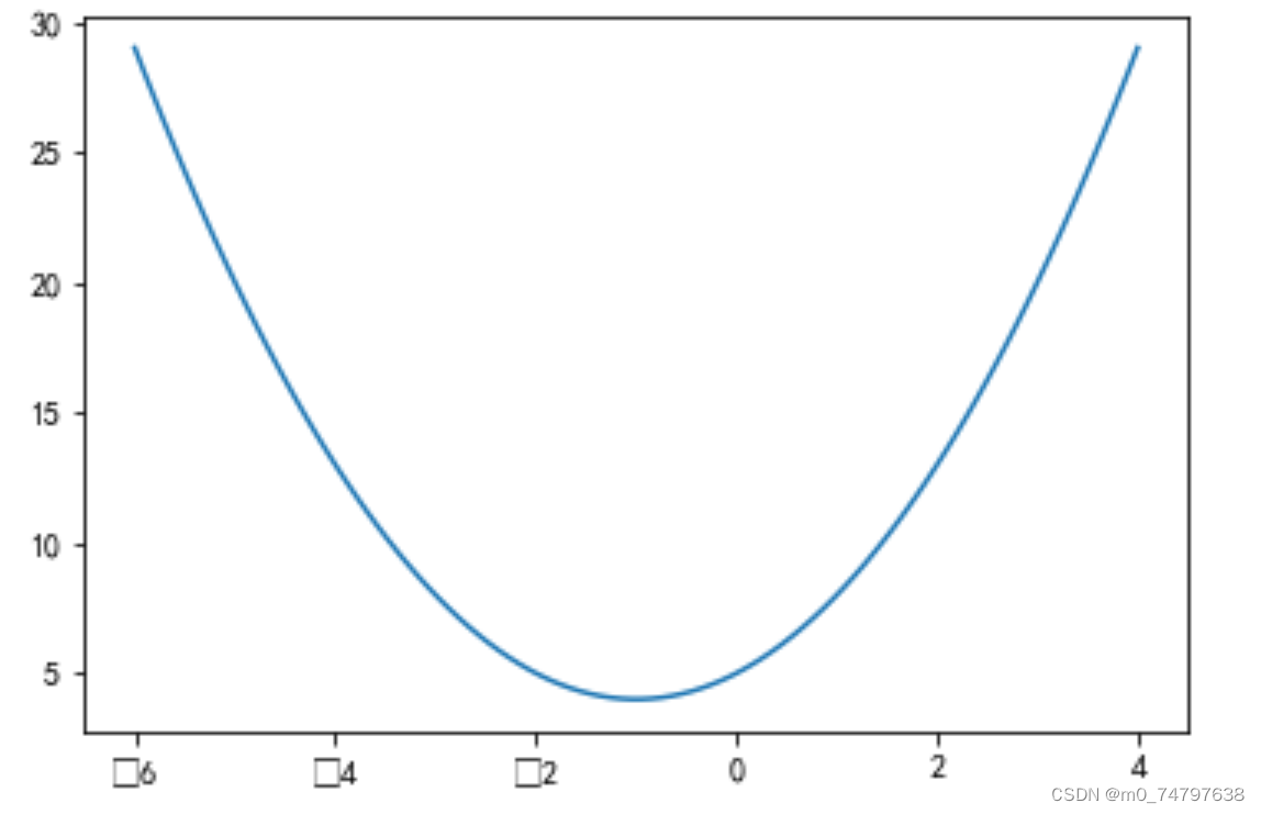
#绘制曲线y=x^2+2x+5
x = np.linspace(-6,4,100)
y = x**2+2*x+5
plt.plot(x,y)

运行结果如下：

 

#参数初始化
x_iter = 3 #x的初值
yita = 0.06 #步长
count = 0 #迭代次数
while True:
    count += 1
    y_last = x_iter ** 2 + x_iter * 2 + 5
    plt.scatter(x_iter,x_iter**2+x_iter*2+5)
    x_iter = x_iter - yita * (2 * x_iter + 2)
    y_next = x_iter ** 2 + x_iter * 2 + 5
    if abs(y_next - y_last)<1e-100:
        break

#绘制曲线y=x^2+2x+5
x = np.linspace(-6,4,100)
y = x**2+2*x+5
plt.plot(x,y)
print('最小值点x=',x_iter,'最小值y=',y_next,'迭代次数n=',count)

运行结果如下：

 

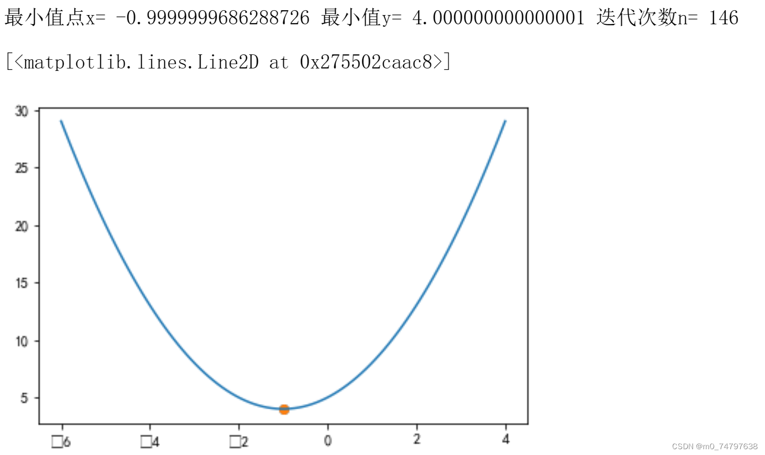
最小值点x= -0.9999999686288726 最小值y= 4.000000000000001 迭代次数n= 146

#参数初始化
x_iter1 = 5 #x的初值
yita1 = 0.05 #步长
count1 = 0 #迭代次数
while count1 < 10:
    count1 += 1
    y_last1 = 2 * x_iter1 ** 2 + x_iter1 * 8 + 15
    x_iter1 = x_iter1 - yita1 * (4 * x_iter1 + 8)
    y_next1 = 2 * x_iter1 ** 2 + x_iter1 * 8 + 15
    if abs(y_next1 - y_last1)<1e-100:
        break
print('最小值点x=',x_iter1,'最小值y=',y_next1,'迭代次数n=',count1)

运行结果为：

最小值点x= -1.2483807232000002 最小值y= 8.12986307451471 迭代次数n= 10

#参数初始化
x_iter2 = 5 #x的初值
yita2 = 0.05 #步长
count2 = 0 #迭代次数
while count2 < 20:
    count2 += 1
    y_last2 = 2 * x_iter2 ** 2 + x_iter2 * 8 + 15
    x_iter2 = x_iter2 - yita2 * (4 * x_iter2 + 8)
    y_next2 = 2 * x_iter2 ** 2 + x_iter2 * 8 + 15
    if abs(y_next2 - y_last2)<1e-100:
        break
print('最小值点x=',x_iter2,'最小值y=',y_next2,'迭代次数n=',count2)

运行结果为：

最小值点x= -1.9192954946775207 最小值y= 7.013026434358692 迭代次数n= 20

#参数初始化
x_iter3 = 5 #x的初值
yita3 = 0.05 #步长
count3 = 0 #迭代次数
while count3 < 1000:
    count3 += 1
    y_last3 = 2 * x_iter3 ** 2 + x_iter3 * 8 + 15
    x_iter3 = x_iter3 - yita3 * (4 * x_iter3 + 8)
    y_next3 = 2 * x_iter3 ** 2 + x_iter3 * 8 + 15
    if abs(y_next3 - y_last3)<1e-100:
        break
print('最小值点x=',x_iter3,'最小值y=',y_next3,'迭代次数n=',count3)

运行结果为：

最小值点x= -1.999999974062572 最小值y= 7.000000000000002 迭代次数n= 87

BGD线性回归代码实现

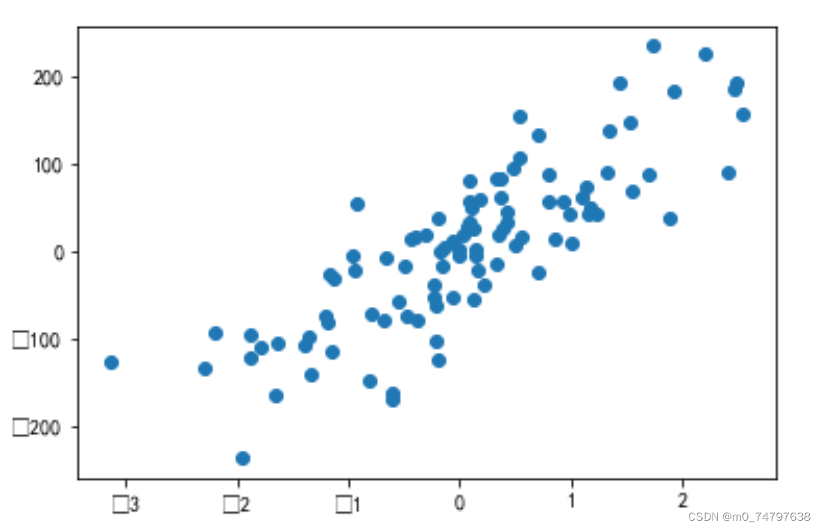
#1.生成回归数据
from sklearn.datasets import make_regression
X,y = make_regression(n_samples=100,n_features=1,noise=50,random_state=8)
plt.scatter(X,y)

运行结果如下：

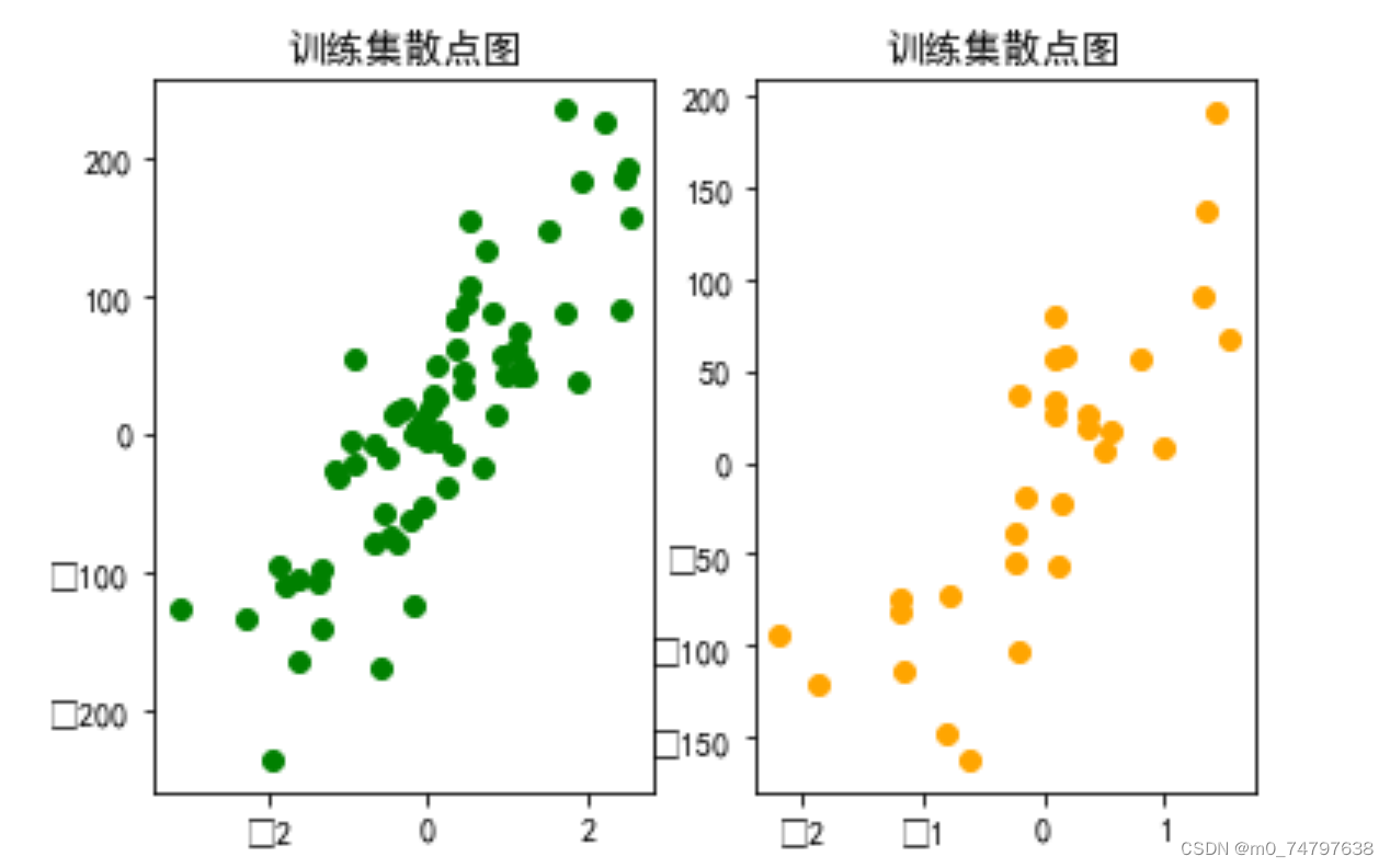
#2.拆分训练集和测试集
from sklearn.model_selection import train_test_split
X_train,X_test,y_train,y_test = train_test_split(X,y,test_size=0.3,random_state=8)
plt.subplot(1,2,1)
plt.scatter(X_train,y_train,c='g')
plt.title("训练集散点图")
plt.subplot(1,2,2)
plt.scatter(X_test,y_test,c='orange')
plt.title("训练集散点图")

 运行结果如下：

#3.利用梯度下降法拟合直线y= wx+b
##3.1 参数初始化
w = 1 #直线斜率
b = -100 #直线截距
lr = 0.001 #学习率learning rate
##3.2 针对参数w和b，先分别计算求和号的值
sum_w = 0
sum_b = 0
for i in range(len(X_train)):
    y_hat = w * X_train[i] + b
    sum_w += (y_train[i] - y_hat) * X_train[i]
    sum_b += y_train[i] - y_hat
##3.3 更新参数w与b的值
w += lr * sum_w
b += lr * sum_b
##3.4 将3.2与3.3重复迭代epochs次
epochs = 1000
for j in range(epochs):
    sum_w = 0
    sum_b = 0
    for i in range(len(X_train)):
        y_hat = w * X_train[i] + b
        sum_w += (y_train[i] - y_hat) * X_train[i]
        sum_b += y_train[i] - y_hat
    #更新参数w与b的值
    w += lr * sum_w
    b += lr * sum_b
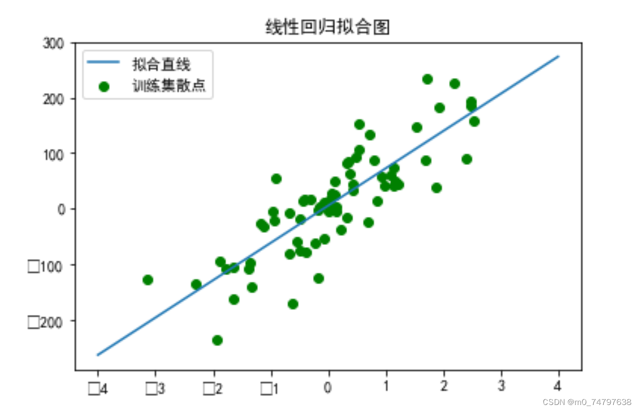
##3.5 将迭代结果可视化
xx = np.linspace(-4,4,100)
yy = w *xx+b
plt.scatter(X_train,y_train,c='g')
plt.plot(xx,yy)
plt.title("线性回归拟合图")
plt.legend(("拟合直线",'训练集散点'))

运行结果如下：

 

##3.6 计算在训练集和测试集上的均方误差
total_loss_train=0
for i in range(len(X_train)):
    y_hat = y_hat = w * X_train[i] + b
    total_loss_train += (y_hat - y_train[i]) ** 2
    
total_loss_test = 0
for i in range(len(X_test)):
    y_hat = y_hat = w * X_test[i] + b
    total_loss_test += (y_hat - y_test[i]) ** 2
    
print(total_loss_train/len(X_train),total_loss_test/len(X_test))

 运行结果为：

[2759.01406036] [2567.72873241]

利用回归模型预测鲍鱼年龄

1 数据集探索性分析

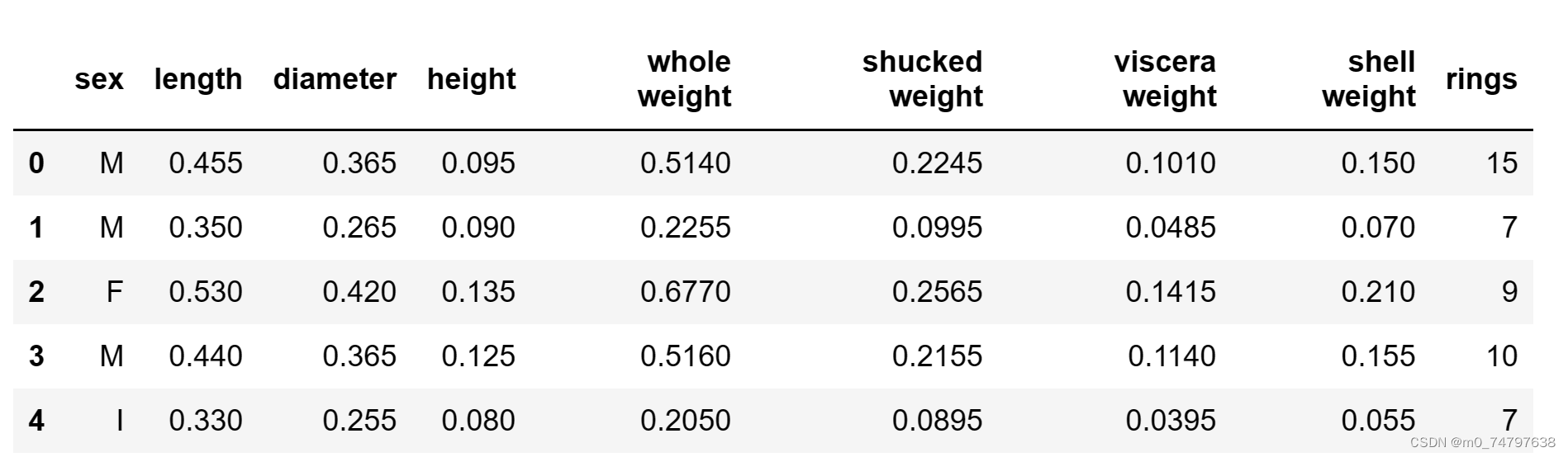
import pandas as pd
data = pd.read_csv("abalone_dataset.csv")
data.head()

 运行结果部分展示：

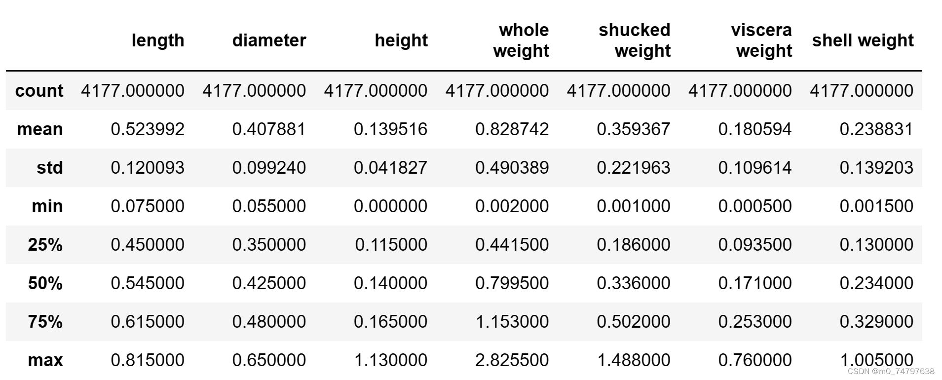
#查看数据集中样本数量和特征数量
data.shape

 运行结果为：

(4177, 9)

data.describe()

运行结果部分展示：

import seaborn as sns
import matplotlib.pyplot as plt
%matplotlib inline

sns.countplot(x="sex",data=data)

运行结果如下：

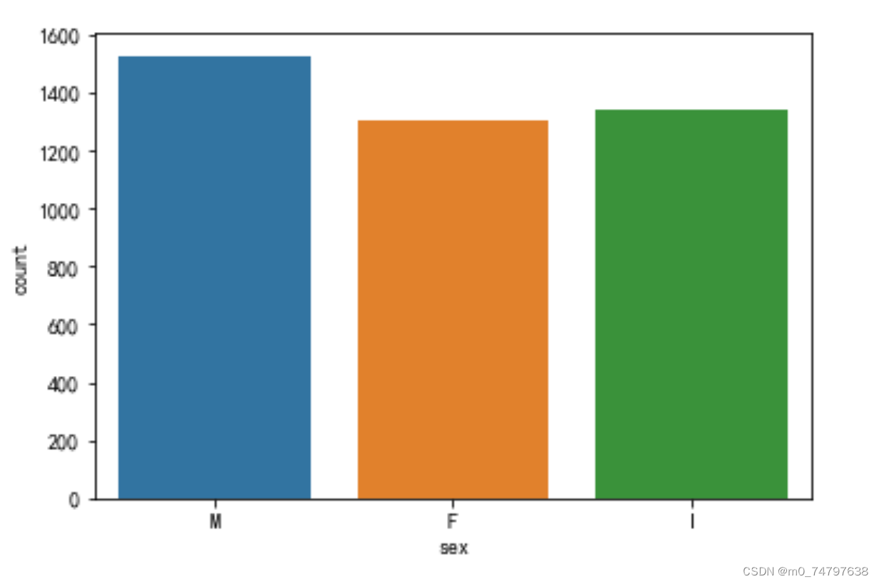
data['sex'].value_counts()

运行结果为：

M    1528
I    1342
F    1307
Name: sex, dtype: int64

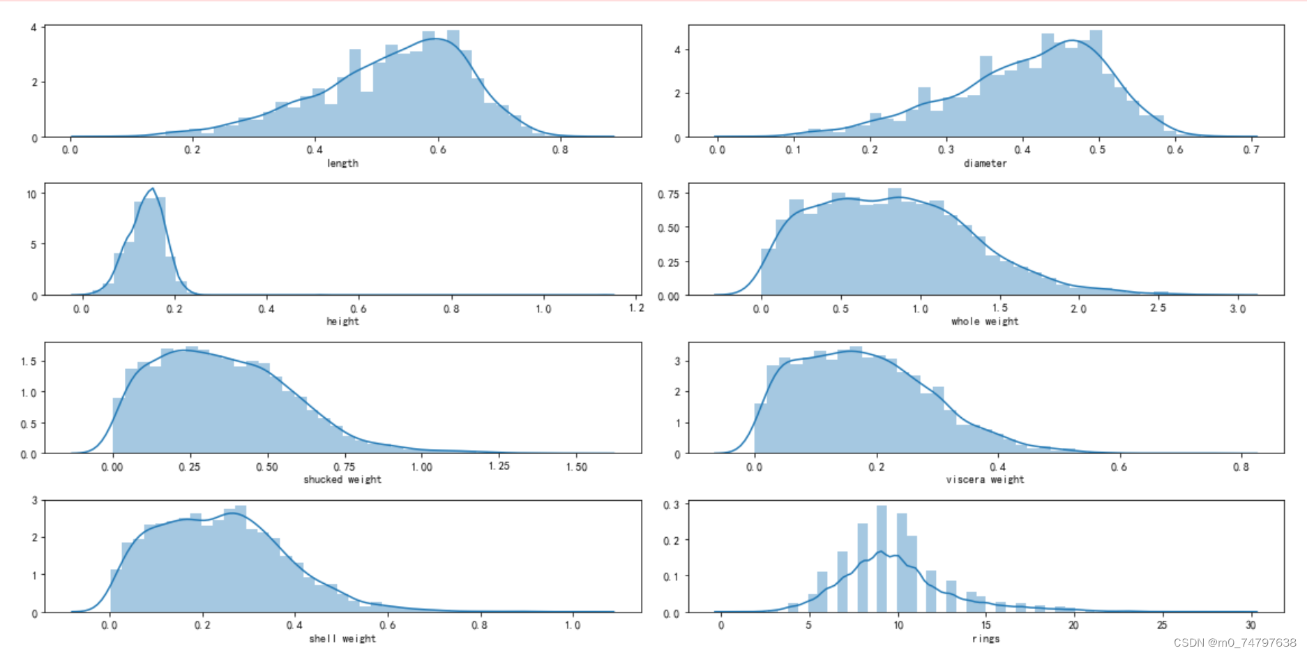
i = 1 #子图记数
plt.figure(figsize=(16,8))
for col in data.columns[1:]:
    plt.subplot(4,2,i)
    i = i + 1
    sns.distplot(data[col])
plt.tight_layout()

运行结果如下：

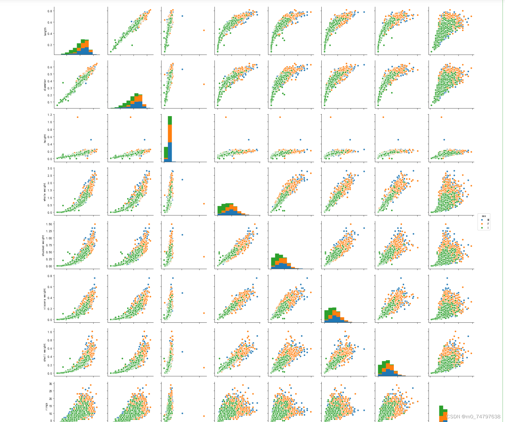
sns.pairplot(data,hue="sex")

 运行结果如下：

 

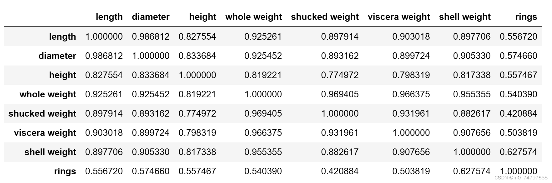
corr_df = data.corr()
corr_df

运行结果如下：

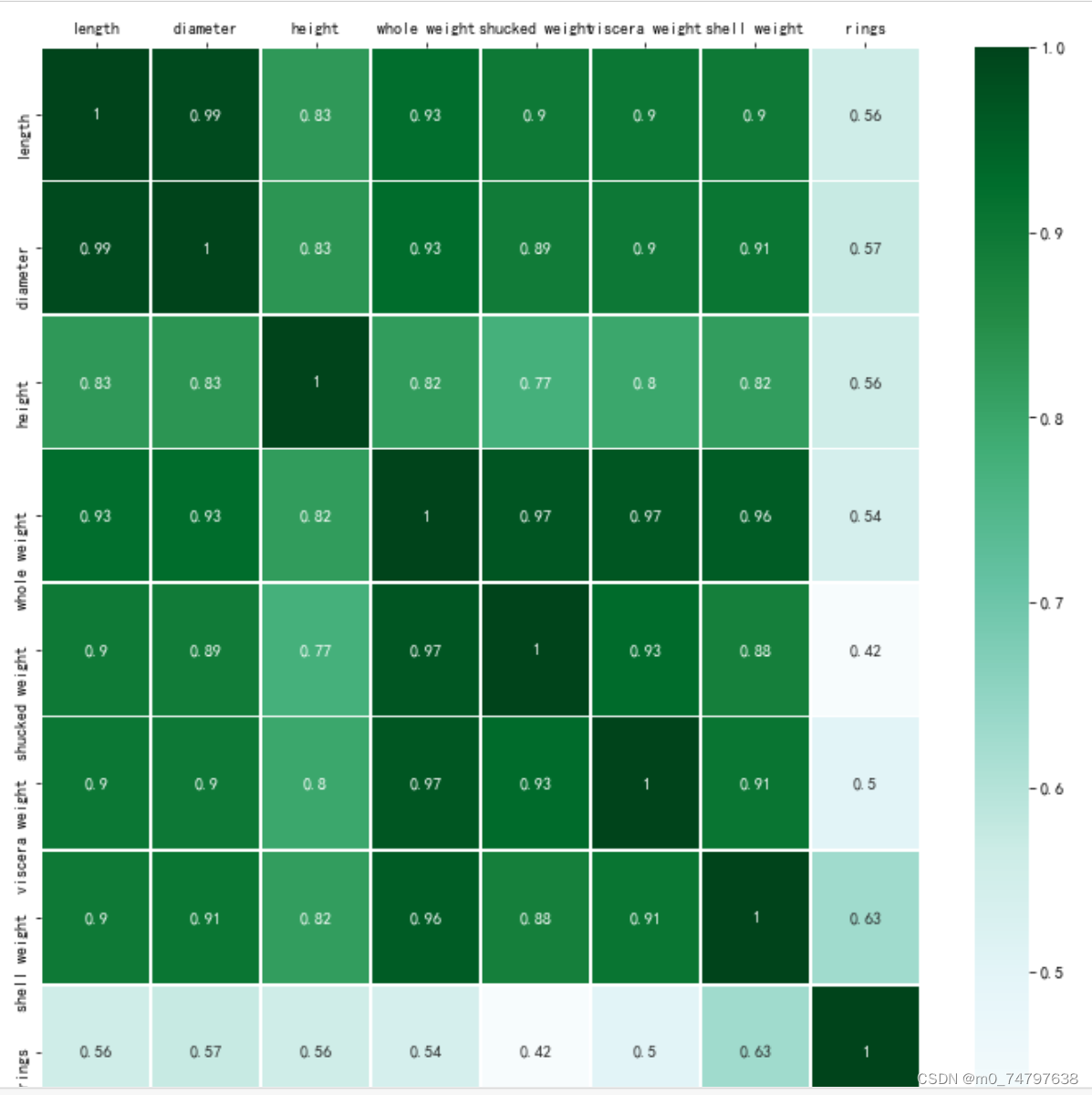
fig, ax=plt.subplots(figsize=(12,12))
##绘制热力图
ax = sns.heatmap(corr_df,linewidths=.5,
                cmap="BuGn",
                annot=True,
                xticklabels=corr_df.columns,
                yticklabels=corr_df.index)
ax.xaxis.set_label_position('top')
ax.xaxis.tick_top()

运行结果如下：

 2鲍鱼数据预处理

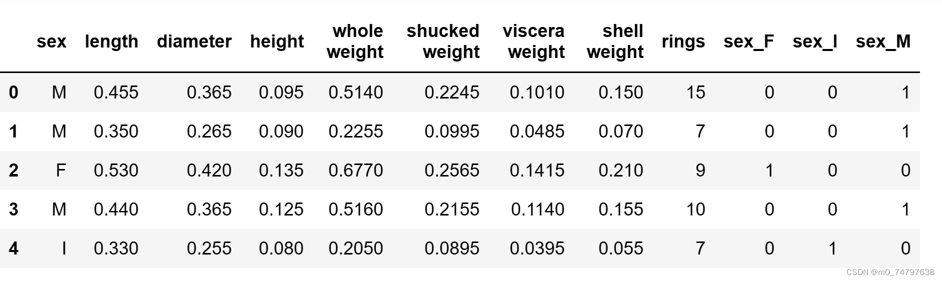
#2.1 对sex的特征进行OneHot编码，便于后续模型纳入哑变量
sex_onehot = pd.get_dummies(data["sex"],prefix="sex")
data[sex_onehot.columns] = sex_onehot
data.head()

运行结果如下：

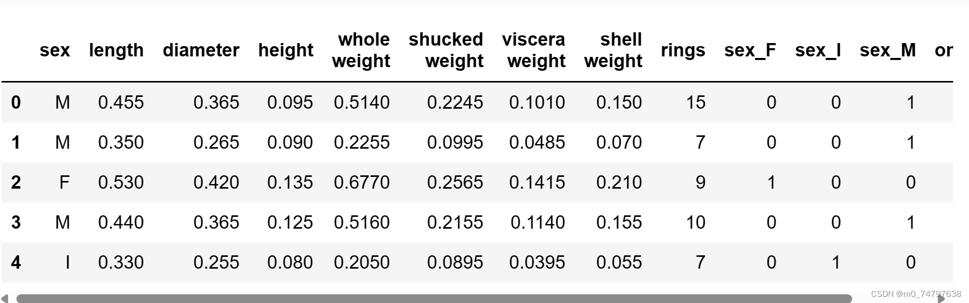
#2.2 添加取值为1的特征
data["ones"]=1
data.head()

运行结果如下：

#2.3 根据鲍鱼环计算年龄
data["age"]=data["rings"]+1.5
data.head()

运行结果如下：

#2.4 筛选特征
y = data["age"]#因变量
features_with_ones = ["length","diameter","height","whole weight","shucked weight","viscera weight","shell weight","sex_F","sex_M","ones"]
features_without_ones = ["length","diameter","height","whole weight","shucked weight","viscera weight","shell weight","sex_F","sex_M"]
X = data[features_with_ones]
#2.5 将鲍鱼数据集划分为训练集和测试集
from sklearn.model_selection import train_test_split
X_train,X_test,y_train,y_test=train_test_split(X,y,test_size=0.2,random_state=111)

3实现线性回归和岭回归

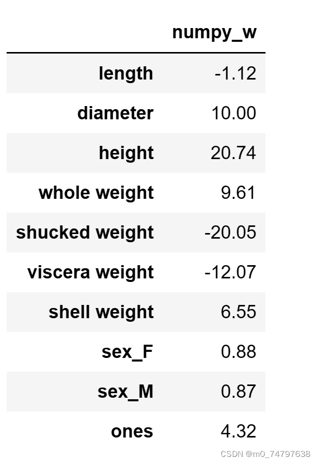
#3.1 使用Numpy实现线性回归
import numpy as np
def linear_regression(X,y):
    w = np.zeros_like(X.shape[1])
    if np.linalg.det(X.T.dot(X))!=0:
        w = np.linalg.inv(X.T.dot(X)).dot(X.T).dot(y)
    return w
w1 = linear_regression(X_train,y_train)
w1 = pd.DataFrame(data=w1,index= X.columns,columns=["numpy_w"])
w1.round(decimals=2)

运行结果如下：

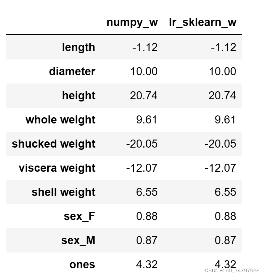
#3.2 使用sklearn实现线性回归
from sklearn.linear_model import LinearRegression
lr = LinearRegression()
lr.fit(X_train[features_without_ones],y_train)
print(lr.coef_)

运行结果为：

[ -1.118146    10.00094599  20.73712616   9.61484657 -20.05079291
 -12.06849193   6.54529076   0.87855188   0.87283083]

w_lr = []
w_lr.extend(lr.coef_)
w_lr.append(lr.intercept_)
w1["lr_sklearn_w"]= w_lr
w1.round(decimals=2)

运行结果如下：

#3.3 使用Numpy实现岭回归（Ridge）
def ridge_regression(X,y,ridge_lambda):
    penalty_matrix = np.eye(X.shape[1])
    penalty_matrix[X.shape[1]-1][X.shape[1]-1]=0
    w=np.linalg.inv(X.T.dot(X)+ridge_lambda*penalty_matrix).dot(X.T).dot(y)
    return w
w2 = ridge_regression(X_train,y_train,1.0)
print(w2)

运行结果：

[  2.30976528   6.72038628  10.23298909   7.05879189 -17.16249532
  -7.2343118    9.3936994    0.96869974   0.9422174    4.80583032]

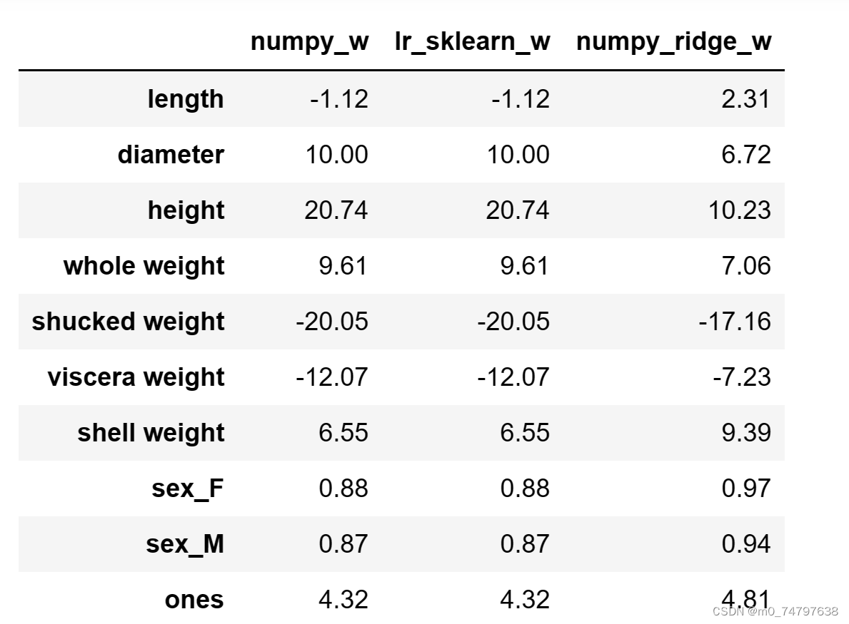
w1["numpy_ridge_w"]=w2
w1.round(decimals=2)

运行结果如下：

#3.4 利用sklearn实现岭回归
from sklearn.linear_model import Ridge
ridge = Ridge(alpha=1.0)
ridge.fit(X_train[features_without_ones],y_train)
w_ridge=[]
w_ridge.extend(ridge.coef_)
w_ridge.append(ridge.intercept_)
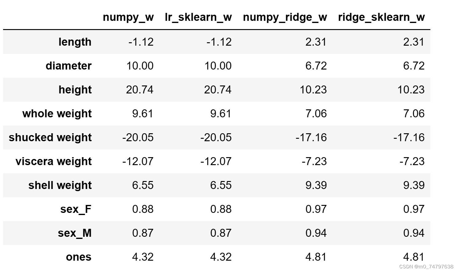
w1["ridge_sklearn_w"]=w_ridge
w1.round(decimals=2)

运行结果如下：

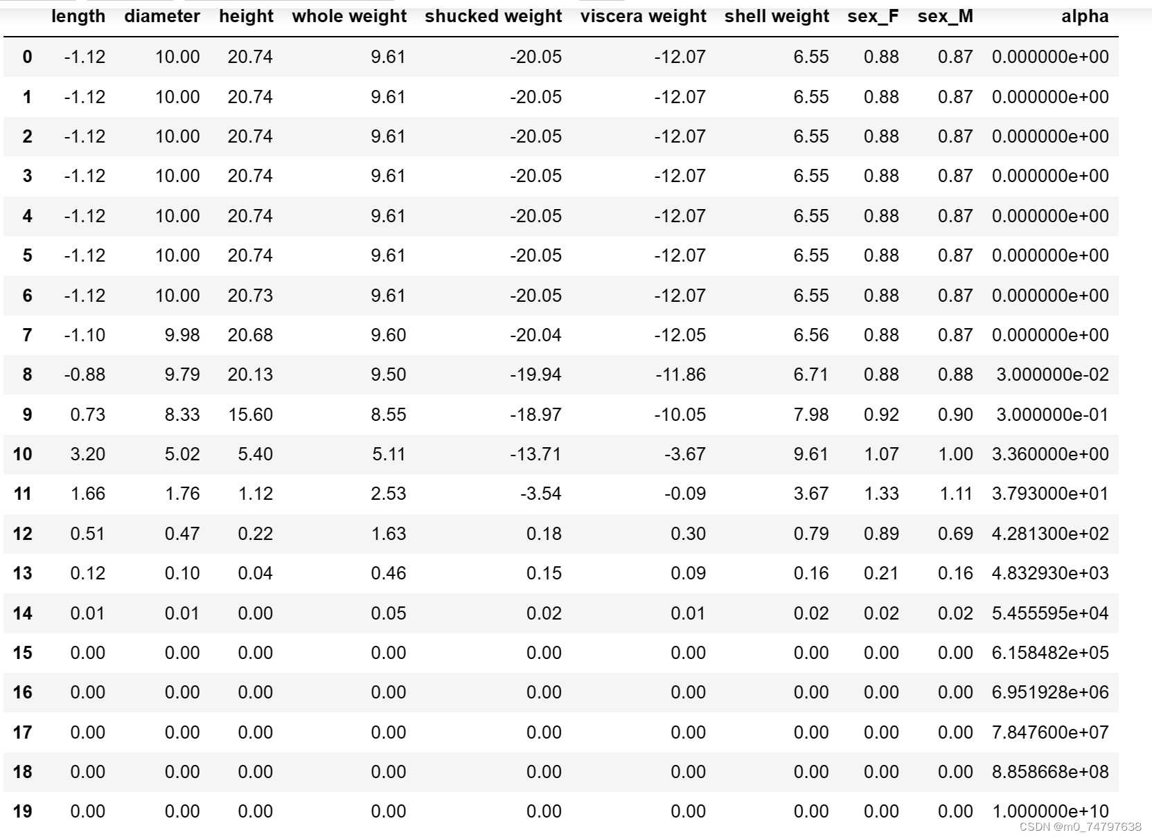
#3.5 岭迹分析
alphas = np.logspace(-10,10,20)
coef = pd.DataFrame()
for alpha in alphas:
    ridge_clf = Ridge(alpha=alpha)
    ridge_clf.fit(X_train[features_without_ones],y_train)
    df = pd.DataFrame([ridge_clf.coef_],columns=X_train[features_without_ones].columns)
    df['alpha'] = alpha
    coef = coef.append(df,ignore_index=True)
coef.round(decimals=2)

运行结果如下：

import matplotlib.pyplot as plt
%matplotlib inline
#绘图
#显示中文和正负号
plt.rcParams['font.sans-serif']=['SimHei','Times New Roman']
plt.rcParams['axes.unicode_minus']=False

plt.rcParams['figure.dpi']=300#分辨率
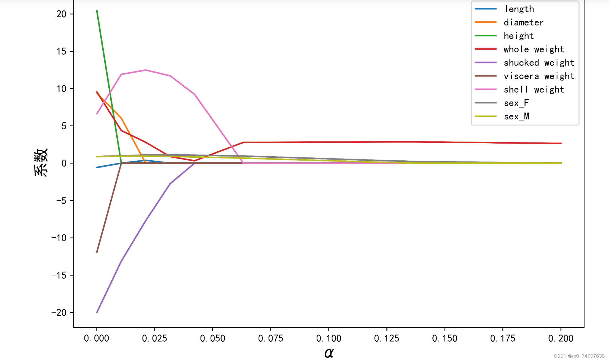
plt.figure(figsize=(9,6))
coef['alpha']=coef['alpha']

for feature in X_train.columns[:-1]:
    plt.plot('alpha',feature,data=coef)
ax=plt.gca()
ax.set_xscale('log')
plt.legend(loc='upper right')
plt.xlabel(r'$\alpha$',fontsize=15)
plt.ylabel('系数',fontsize=15)

 运行结果如下：

4使用LASSO构建鲍鱼年龄预测模型

from sklearn.linear_model import Lasso
lasso = Lasso(alpha=0.01)
lasso.fit(X_train[features_without_ones],y_train)
print(lasso.coef_)
print(lasso.intercept_)

运行结果为：

[  0.           6.37435514   0.           4.46703234 -13.44947667
  -0.          11.85934842   0.98908791   0.93313403]
6.500338023591297

#LASSO的正则化路径
coef = pd.DataFrame()
for alpha in np.linspace(0.0001,0.2,20):
    lasso_clf = Lasso(alpha=alpha)
    lasso_clf.fit(X_train[features_without_ones],y_train)
    df = pd.DataFrame([lasso_clf.coef_],columns=X_train[features_without_ones].columns)
    df['alpha']=alpha
    coef = coef.append(df,ignore_index=True)
coef.head()
#绘图
plt.figure(figsize=(9,6),dpi=600)
for feature in X_train.columns[:-1]:
    plt.plot('alpha',feature,data=coef)
plt.legend(loc='upper right')
plt.xlabel(r'$\alpha$',fontsize=15)
plt.ylabel('系数',fontsize=15)
plt.show()

运行结果如下：

 5鲍鱼年龄预测模型效果评估

from sklearn.metrics import mean_squared_error
from sklearn.metrics import mean_absolute_error
from sklearn.metrics import r2_score
#MAE
y_test_pred_lr = lr.predict(X_test.iloc[:,:-1])
print(round(mean_absolute_error(y_test,y_test_pred_lr),4))

y_test_pred_ridge = ridge.predict(X_test[features_without_ones])
print(round(mean_absolute_error(y_test,y_test_pred_ridge),4))

y_test_pred_lasso = lasso.predict(X_test[features_without_ones])
print(round(mean_absolute_error(y_test,y_test_pred_lasso),4))

 运行结果为：

1.6016
1.5984
1.6402

#MSE
y_test_pred_lr = lr.predict(X_test.iloc[:,:-1])
print(round(mean_squared_error(y_test,y_test_pred_lr),4))

y_test_pred_ridge = ridge.predict(X_test[features_without_ones])
print(round(mean_squared_error(y_test,y_test_pred_ridge),4))

y_test_pred_lasso = lasso.predict(X_test[features_without_ones])
print(round(mean_squared_error(y_test,y_test_pred_lasso),4))

运行结果为：

5.3009
4.959
5.1

#R2系数
print(round(r2_score(y_test,y_test_pred_lr),4))
print(round(r2_score(y_test,y_test_pred_ridge),4))
print(round(r2_score(y_test,y_test_pred_lasso),4))

运行结果为：

0.5257
0.5563
0.5437

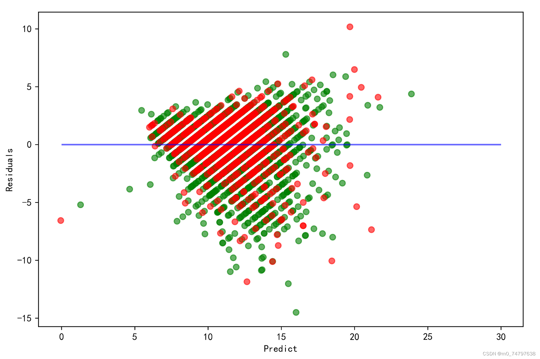
#5.2 残差图
plt.figure(figsize=(9,6),dpi=600)
y_train_pred_ridge = ridge.predict(X_train[features_without_ones])
plt.scatter(y_train_pred_ridge,y_train_pred_ridge - y_train,c="g",alpha=0.6)
plt.scatter(y_test_pred_ridge,y_test_pred_ridge - y_test,c="r",alpha=0.6)
plt.hlines(y=0,xmin=0,xmax=30,colors="b",alpha=0.6)
plt.ylabel("Residuals")
plt.xlabel("Predict")

运行结果如下：