对 SPY 和 IWM 之间的日内均值回归配对策略进行回测

对 SPY 和 IWM 之间的日内均值回归配对策略进行回测

在本文中，我们将讨论我们的第一个日内交易策略。它将使用经典的交易理念，即“交易对”。在这种情况下，我们将利用两只交易所交易基金(ETF)，SPY和IWM，它们在纽约证券交易所 (NYSE) 交易，并分别试图代表美国股票市场指数，即标准普尔 500 指数和罗素 2000 指数。

该策略通过做多一只 ETF 并做空一定数量的 ETF 来大致在 ETF 对之间创建“价差”。多头与空头的比率可以通过多种方式定义，例如利用统计协整时间序列技术。在这种情况下，我们将通过滚动线性回归计算 SPY 和 IWM 之间的对冲比率。这将使我们能够在 SPY 和 IWM 之间创建“价差”，并将其标准化为z 分数。当 z 分数超过某些阈值时，将生成交易信号，因为我们相信价差将恢复到平均值。

该策略的原理是 SPY 和 IWM 大致描述了相同的情况，即一组大型和小型美国公司的经济状况。前提是，如果采用价格差，那么它应该是均值回归的，因为虽然“局部”（时间）事件可能会分别影响 S&P500 或 Russell 2000 指数（例如小型/大型股差异、重新平衡日期或大宗交易），但两者的长期价格序列可能会协整。

策略

该策略按以下步骤进行：

1. 数据- SPY 和 IWM 的 1 分钟条形图是从 2007 年 4 月到 2014 年 2 月获得的。
2. 处理- 数据正确对齐，缺失的条形被相互丢弃。
3. 价差- 两只 ETF 之间的对冲比率是通过滚动线性回归计算得出的。这被定义为𝛽回归系数使用*回溯窗口，*该窗口向前移动 1 条并重新计算回归系数。因此对冲比率𝛽我，用于酒吧𝑏我跨点计算𝑏我−1−钾到𝑏我−1回顾钾酒吧。
4. Z 分数- 点差的标准分数以通常的方式计算。这意味着减去点差的（样本）平均值并除以点差的（样本）标准差。这样做的理由是使阈值参数更易于理解，因为 z 分数是无量纲量。我们故意在计算中引入了前瞻偏差，以显示它有多么微妙。试着留意它！
5. 交易- 当负 z 分数低于预定（或优化后）阈值时，会产生多头信号，而空头信号则相反。当绝对 z 分数低于另一个阈值时，会产生退出信号。对于此策略，我（有点随意地）选择了绝对进入阈值|是|=2退出门槛为|是|=1. 假设价差呈现均值回归行为，则有望捕捉到这种关系并提供积极的表现。

深入了解该策略的最佳方式可能是实际实施它。以下部分描述了用于实施此均值回归策略的完整 Python 代码（单个文件）。为了帮助理解，我对代码进行了大量的注释。

Python 实现

与所有 Python/pandas 教程一样，需要按照本教程中的说明设置 Python 研究环境。设置完成后，第一项任务是导入必要的 Python 库。此回测需要matplotlib和pandas 。

我使用的具体库版本如下：

• Python - 3.8
• NumPy-1.20
• 熊猫-1.3
• matplotlib-3.4
• 统计模型-0.12

让我们继续导入库：

# mr_spy_iwm.py

import matplotlib.pyplot as plt
import numpy as np
import os, os.path
import pandas as pd
import seaborn as sns

import statsmodels.api as sm
from statsmodels.regression.rolling import RollingOLS

sns.set_style("darkgrid")

以下函数create_pairs_dataframe导入两个包含两个符号的日内条形图的 CSV 文件。在我们的例子中，这两个符号是 SPY 和 IWM。然后，它创建一个单独的数据框pairs，使用两个原始文件的索引。由于它们的时间戳可能由于错过交易和错误而不同，因此这可以保证我们将获得匹配的数据。这是使用 pandas 等数据分析库的主要好处之一。“样板”代码以非常高效的方式为我们处理。

# mr_spy_iwm.py

def create_pairs_dataframe(datadir, symbols):
    """
    Creates a pandas DataFrame containing the closing price
    of a pair of symbols based on CSV files containing a datetime
    stamp and OHLCV data.

    Parameters
    ----------
    datadir : `str`
        Directory location of CSV files containing OHLCV intraday data.
    symbols : `tup`
        Tuple containing ticker symbols as `str`.

    Returns
    -------
    pairs : `pd.DataFrame`
        A DataFrame containing Close price for SPY and IWM. Index is a 
        Datetime object.
    """
    # Open the individual CSV files and read into pandas DataFrames 
    # using the first column as an index and col_names as the headers
    
    print("Importing CSV data...")
    col_names = ['datetime','open','high','low','close', 'volume', 'na']
    sym1 = pd.read_csv(
        os.path.join(datadir, '%s.csv' % symbols[0]),
        header=0,
        index_col=0,
        names=col_names
    )
    sym2 = pd.read_csv(
        os.path.join(datadir, '%s.csv' % symbols[1]),
        header=0,
        index_col=0,
        names=col_names
    )

    # Create a pandas DataFrame with the close prices of each symbol
    # correctly aligned and dropping missing entries
    print("Constructing dual matrix for %s and %s..." % symbols)
    pairs = pd.DataFrame(index=sym1.index)
    pairs['%s_close' % symbols[0].lower()] = sym1['close']
    pairs['%s_close' % symbols[1].lower()] = sym2['close']
    pairs.index = pd.to_datetime(pairs.index)
    pairs = pairs.dropna()
    return pairs

下一步是执行 SPY 和 IWM 之间的滚动线性回归。在这种情况下，IWM 是预测因子（“x”），SPY 是响应（“y”）。我已设置 100 条的默认回溯窗口。如上所述，这是策略的一个参数。为了使策略被视为稳健，我们理想情况下希望将回报概况（或其他绩效衡量标准）视为回溯期的凸函数。因此，在代码的后期阶段，我们将通过在一定范围内改变回溯期来进行敏感性分析。

在SPY-IWM 的线性回归模型中计算出滚动贝塔pairs系数后，我们将其添加到DataFrame 中并删除空行。这构成了第一组与回溯大小相等的条形图，作为修剪指标。然后，我们创建两个 ETF 的价差，作为 SPY 和−𝛽我IWM 单位。显然，这不是现实情况，因为我们采用的是 IWM 的分数，这在实际实施中是不可能的。

最后，我们创建价差的 z 分数，该分数通过减去价差的平均值并用价差的标准差进行归一化来计算。请注意，这里出现了一个相当微妙的前瞻偏差。我故意把它留在代码中，因为我想强调在研究中犯这样的错误是多么容易。平均值和标准差是针对整个价差时间序列计算的。如果这是为了反映真实的历史准确性，那么这些信息将无法获得，因为它隐含地利用了未来信息。因此，我们应该使用滚动平均值和标准差来计算 z 分数。

# mr_spy_iwm.py

def calculate_spread_zscore(pairs, symbols, lookback=100):
    """
    Creates a hedge ratio between the two symbols by calculating
    a rolling linear regression with a defined lookback period. This
    is then used to create a z-score of the 'spread' between the two
    symbols based on a linear combination of the two.

    Parameters
    ----------
    pairs : `pd.DataFrame`
        A DataFrame containing Close price for SPY and IWM. Index is a 
        Datetime object.
    symbols : `tup`
        Tuple containing ticker symbols as `str`.
    lookback : `int`, optional (default: 100)
        Lookback preiod for rolling linear regression.

    Returns
    -------
    pairs : 'pd.DataFrame'
        Updated DataFrame containing the spread and z score between
        the two symbols based on the rolling linear regression.    
    """

    # Use the statsmodels Rolling Ordinary Least Squares method to fit
    # a rolling linear regression between the two closing price time series
    print("Fitting the rolling Linear Regression...")

    model = RollingOLS(
        endog=pairs['%s_close' % symbols[0].lower()],
        exog=sm.add_constant(pairs['%s_close' % symbols[1].lower()]),
        window=lookback
    )
    rres = model.fit()
    params = rres.params.copy()
    
    
    # Construct the hedge ratio and eliminate the first 
    # lookback-length empty/NaN period
    pairs['hedge_ratio'] = params['iwm_close']
    pairs.dropna(inplace=True)

    # Create the spread and then a z-score of the spread
    print("Creating the spread/zscore columns...")
    pairs['spread'] = (
        pairs['spy_close'] - pairs['hedge_ratio']*pairs['iwm_close']
    )
    pairs['zscore'] = (
        pairs['spread'] - np.mean(pairs['spread']))/np.std(pairs['spread']
    )
    return pairs

交易信号create_long_short_market_signals已创建。这些信号通过以下方式计算：当 z 分数负向超过负 z 分数时做多价差，当 z 分数正向超过正 z 分数时做空价差。当 z 分数的绝对值小于或等于另一个（幅度较小的）阈值时，发出退出信号。

为了实现这种情况，必须知道每个条形图的策略是“进入”市场还是“退出”市场。long_market和short_market是两个变量，用于跟踪多头和空头市场头寸。不幸的是，与矢量化方法相比，以迭代方式编码要简单得多，因此计算速度很慢。尽管 1 分钟的条形图需要每个 CSV 文件约 700,000 个数据点，但在我的旧台式机上计算速度仍然相对较快！

要迭代 pandas DataFrame（诚然这不是一个常见操作），必须使用该iterrows方法，该方法提供了一个可以迭代的生成器：

# mr_spy_iwm.py

def create_long_short_market_signals(
        pairs, symbols, z_entry_threshold=2.0, z_exit_threshold=1.0
    ):
    """
    Create the entry/exit signals based on the exceeding of z_entry_threshold
    for entering a position and falling below z_exit_threshold for exiting
    a position.

    Parameters
    ----------
    pairs : `pd.DataFrame`
        Updated DataFrame containing the close price, spread and z score
        between the two symbols.
    symbols : `tup`
        Tuple containing ticker symbols as `str`.
    z_entry_threshold : `float`, optional (default:2.0)
        Z Score threshold for market entry. 
    z_exit_threshold : `float`, optional (default:1.0)
        Z Score threshold for market exit.

    Returns
    -------
    pairs : `pd.DataFrame`
        Updated DataFrame containing long, short and exit signals.
    """

    # Calculate when to be long, short and when to exit
    pairs['longs'] = (pairs['zscore'] <= -z_entry_threshold)*1.0
    pairs['shorts'] = (pairs['zscore'] >= z_entry_threshold)*1.0
    pairs['exits'] = (np.abs(pairs['zscore']) <= z_exit_threshold)*1.0

    # These signals are needed because we need to propagate a
    # position forward, i.e. we need to stay long if the zscore
    # threshold is less than z_entry_threshold by still greater
    # than z_exit_threshold, and vice versa for shorts.
    pairs['long_market'] = 0.0
    pairs['short_market'] = 0.0

    # These variables track whether to be long or short while
    # iterating through the bars
    long_market = 0
    short_market = 0

    # Calculates when to actually be "in" the market, i.e. to have a
    # long or short position, as well as when not to be.
    # Since this is using iterrows to loop over a dataframe, it will
    # be significantly less efficient than a vectorised operation,
    # i.e. slow!
    print("Calculating when to be in the market (long and short)...")
    for i, b in enumerate(pairs.iterrows()):
        # Calculate longs
        if b[1]['longs'] == 1.0:
            long_market = 1            
        # Calculate shorts
        if b[1]['shorts'] == 1.0:
            short_market = 1
        # Calculate exists
        if b[1]['exits'] == 1.0:
            long_market = 0
            short_market = 0
        # This directly assigns a 1 or 0 to the long_market/short_market
        # columns, such that the strategy knows when to actually stay in!
        pairs.iloc[i]['long_market'] = long_market
        pairs.iloc[i]['short_market'] = short_market
    return pairs

在此阶段，我们已更新pairs以包含实际的多头/空头信号，这使我们能够确定是否需要进入市场。现在我们需要创建一个投资组合来跟踪头寸的市场价值。第一个任务是创建一个positions结合多头和空头信号的列。这将包含来自（1，0，−1）， 和1代表多头/市场仓位，0表示没有头寸（应该退出）并且−1表示空头/市场仓位。sym1和sym2列表示每根柱线收盘时 SPY 和 IWM 仓位的市场价值。

创建 ETF 市场价值后，我们会将它们相加，以在每条柱状图末尾得出总市场价值。然后，pct_change该 Series 对象的方法会将其转换为回报流。后续代码行会清除不良条目（NaN 和 inf 元素），最后计算完整的权益曲线。

# mr_spy_iwm.py

def create_portfolio_returns(pairs, symbols):
    """
    Creates a portfolio pandas DataFrame which keeps track of
    the account equity and ultimately generates an equity curve.
    This can be used to generate drawdown and risk/reward ratios.
    
    Parameters
    ----------
    pairs : `pd.DataFrame`
        Updated DataFrame containing the close price, spread and z score
        between the two symbols and the long, short and exit signals.
    symbols : `tup`
        Tuple containing ticker symbols as `str`.

    Returns
    -------
    portfolio : 'pd.DataFrame'
        A DataFrame with datetime index from the pairs DataFrame, positions,
        total market value and returns.
    """
    
    # Convenience variables for symbols
    sym1 = symbols[0].lower()
    sym2 = symbols[1].lower()

    # Construct the portfolio object with positions information
    # Note the minuses to keep track of shorts!
    print("Constructing a portfolio...")
    portfolio = pd.DataFrame(index=pairs.index)
    portfolio['positions'] = pairs['long_market'] - pairs['short_market']
    portfolio[sym1] = -1.0 * pairs['%s_close' % sym1] * portfolio['positions']
    portfolio[sym2] = pairs['%s_close' % sym2] * portfolio['positions']
    portfolio['total'] = portfolio[sym1] + portfolio[sym2]

    # Construct a percentage returns stream and eliminate all 
    # of the NaN and -inf/+inf cells
    print("Constructing the equity curve...")
    portfolio['returns'] = portfolio['total'].pct_change()
    portfolio['returns'].fillna(0.0, inplace=True)
    portfolio['returns'].replace([np.inf, -np.inf], 0.0, inplace=True)
    portfolio['returns'].replace(-1.0, 0.0, inplace=True)

    # Calculate the full equity curve
    portfolio['returns'] = (portfolio['returns'] + 1.0).cumprod()
    return portfolio

该__main__函数将所有内容整合在一起。盘中 CSV 文件位于路径中datadir。请确保修改以下代码以指向您的特定目录。

为了确定策略对回溯期的敏感度，有必要计算一系列回溯的绩效指标。我选择了投资组合的最终总回报率作为绩效衡量标准，回溯范围为[50，200]以 10 为增量。您可以在以下代码中看到，前面的函数被包装在for这个范围内的循环中，其他阈值保持不变。最后一项任务是使用 matplotlib 创建回顾与回报的折线图：

# mr_spy_iwm.py

if __name__ == "__main__":
    datadir = '/your/path/to/data/'  # Change this to reflect your data path!
    symbols = ('SPY', 'IWM')

    lookbacks = range(50, 210, 10)
    returns = []

    # Adjust lookback period from 50 to 200 in increments
    # of 10 in order to produce sensitivities
    for lb in lookbacks: 
        print("Calculating lookback=%s..." % lb)
        pairs = create_pairs_dataframe(datadir, symbols)
        pairs = calculate_spread_zscore(pairs, symbols, lookback=lb)
        pairs = create_long_short_market_signals(
            pairs, symbols, z_entry_threshold=2.0, z_exit_threshold=1.0
        )
        portfolio = create_portfolio_returns(pairs, symbols)
        returns.append(portfolio.iloc[-1]['returns'])

    print("Plot the lookback-performance scatterchart...")
    plt.plot(lookbacks, returns, '-o')
    plt.show()

现在可以看到回溯期与回报的图表。请注意，在回溯等于 110 条时有一个“全局”最大值。如果我们看到回溯与回报无关的情况，那么这将引起关注：

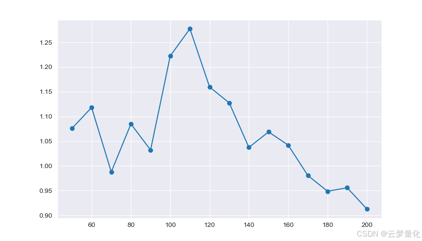
SPY-IWM 线性回归对冲比率回顾期敏感性分析

如果没有向上倾斜的股权曲线，那么任何回溯测试文章都是不完整的！因此，如果您希望绘制累计收益与时间的曲线，则可以使用以下代码，该代码将绘制从回溯参数研究中生成的最终投资组合。您需要根据要可视化的图表来选择回溯。该图表还绘制了 SPY 在同一时期的收益，以帮助进行比较：

 #mr_spy_iwm.py

    # This is still within the main function
    print("Plotting the performance charts...")
    fig = plt.figure()

    ax1 = fig.add_subplot(211,  ylabel='%s growth (%%)' % symbols[0])
    (pairs['%s_close' % symbols[0].lower()].pct_change()+1.0).cumprod().plot(ax=ax1, color='r', lw=2.)

    ax2 = fig.add_subplot(212, ylabel='Portfolio value growth (%%)')
    portfolio['returns'].plot(ax=ax2, lw=2.)

    plt.show()

以下股权曲线图的回顾期为 100 天：

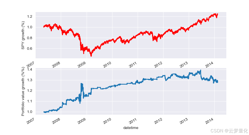
SPY-IWM 均值回归策略投资组合权益曲线

请注意，SPY 在 2009 年金融危机期间的下跌幅度很大。该策略在此阶段也经历了一段波动期。还请注意，由于 SPY 在此期间的强烈趋势性（反映了标准普尔 500 指数），其表现在去年有所恶化。

请注意，在计算价差的 z 分数时，我们仍然必须考虑前瞻偏差。此外，所有这些计算都是在没有交易成本的情况下进行的。一旦考虑到这些因素，该策略的表现肯定会非常糟糕。费用、买卖价差和滑点目前都未考虑在内。此外，该策略以 ETF 的零碎单位进行交易，这也非常不现实。

转存中…(img-DmAD6tBp-1729221920090)]SPY-IWM 均值回归策略投资组合权益曲线

请注意，SPY 在 2009 年金融危机期间的下跌幅度很大。该策略在此阶段也经历了一段波动期。还请注意，由于 SPY 在此期间的强烈趋势性（反映了标准普尔 500 指数），其表现在去年有所恶化。

请注意，在计算价差的 z 分数时，我们仍然必须考虑前瞻偏差。此外，所有这些计算都是在没有交易成本的情况下进行的。一旦考虑到这些因素，该策略的表现肯定会非常糟糕。费用、买卖价差和滑点目前都未考虑在内。此外，该策略以 ETF 的零碎单位进行交易，这也非常不现实。

在后面的文章中，我们将创建一个更加复杂的事件驱动回测器，它将考虑到这些因素，并让我们对我们的权益曲线和绩效指标更加有信心。