SIR

疫情数据预测

疫情来势汹汹，在家闲着无聊的我事先预备好疫情数据，准备预测一下疫情未来的走势。

载入数据

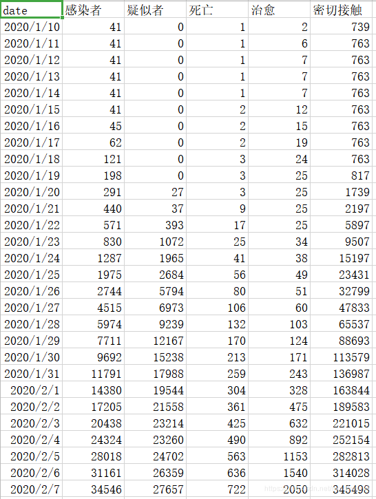
获取事先已经爬取好的疫情数据，通过作图分析，发现病毒蔓延的实在疯狂，从未料到2020年的大门被一场巨大的灾难打开。

import matplotlib.pyplot as plt
import numpy as np
import pandas as pd
from sklearn.preprocessing import PolynomialFeatures
from sklearn.linear_model import LinearRegression

# 载入数据
data = pd.read_csv('data.csv')
#print(data)
data["现有感染者"] = data["感染者"] - data["死亡"] - data["治愈"]
data['发展'] = np.arange(1,34)
print(data)

数据大概长这样子：

分析数据

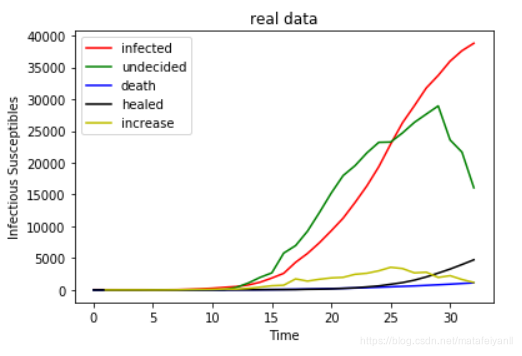
画出疫情走势图

# 数据作图
fig = plt.figure()
plt.subplot(111)
plt.plot(data["现有感染者"], "-r", label = "infected")
plt.plot(data["疑似者"], "-g", label = "undecided")
plt.plot(data["死亡"], "-b", label = "death")
plt.plot(data["治愈"], "-k", label = "healed")
plt.plot(data["现有感染者"]-data["现有感染者"].shift(1), "-y", label = "increase")
plt.legend(loc = 0)
plt.title("real data")
plt.xlabel("Time")
plt.ylabel("Infectious Susceptibles")
plt.show()

模型稍稍有点复杂，但是数据量又有点小，那就用多项式回归来预测试试看吧

构建模型

可以通过不断调节多项式的特征来改变拟合程度

def logical_model(x_data,y_data,degree):
    # 定义多项式回归,degree的值可以调节多项式的特征
    poly_reg  = PolynomialFeatures(degree) 
    # 特征处理
    x_poly = poly_reg.fit_transform(x_data)
    # 定义回归模型
    lin_reg = LinearRegression()
    # 训练模型
    lin_reg.fit(x_poly, y_data)
    return lin_reg,poly_reg

训练模型

训练模型并作图

Infected_model,Infected_reg = logical_model(npdata[:,-1,np.newaxis],npdata[:,1,np.newaxis],5)
Undecided_model,Undecided_reg = logical_model(npdata[:,-1,np.newaxis],npdata[:,2,np.newaxis],5)
Death_model,Death_reg = logical_model(npdata[:,-1,np.newaxis],npdata[:,3,np.newaxis],4)
Health_model,Health_reg = logical_model(npdata[:,-1,np.newaxis],npdata[:,4,np.newaxis],6)

test = np.linspace(0,60,1000)[:,np.newaxis]
#print(Infected_test)
figure = plt.figure()
plt.ylim(0,50000)
plt.plot(test,Infected_model.predict(Infected_reg.fit_transform(test)),"-r",label = "infected")
plt.plot(test,Undecided_model.predict(Undecided_reg.fit_transform(test)),"-g",label = "undecided")
plt.plot(test,Death_model.predict(Death_reg.fit_transform(test)),"-b", label = "death")
plt.plot(test,Health_model.predict(Health_reg.fit_transform(test)), "-k", label = "healed")
plt.legend(loc = 0)
plt.title("prediction data")
plt.xlabel("Time")
plt.ylabel("Infectious Susceptibles")
plt.show()

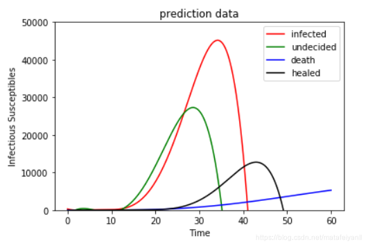
啊，疫情的下降速率有点快哈，那也不错，如果疫情控制得当的话，未尝不是一件好事呢。

SIR模型

考虑到传染病预测模型SIR，便了解了一番
SIR模型是一种传播模型，是信息传播过程的抽象描述。
SIR模型是传染病模型中最经典的模型，其中S表示易感者，I表示感染者，R表示移除者。

S：Susceptible，易感者
I：Infective，感染者
R：Removal，移除者

一般认为人群总数N是不变的，分为易感人群，感染者和治愈者，于是有

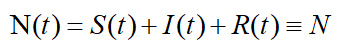
关于SIR的微分方程

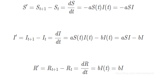
a为感染率，b为恢复率
路径图如下：
S------(aSI)------> I ------(bI)-----> R

SIR代码实现

那就用SIR模型来预测一下吧

import scipy.integrate as spi
a = 5e-6   #感染率
b = 0.04  #恢复率
TS = 1.0    
ND = 60.0
S0 = 60000   #易感者
I0 = 41    #感染者
INPUT = [S0, I0, 0.0]


# 模型的差分方程
def diff_eqs(INP, t):
    Y = np.zeros((3)) 
    V = INP
    #print(V)
    Y[0] = -a * V[0] * V[1]
    Y[1] = a * V[0] * V[1] - b * V[1]
    Y[2] = b * V[1]
    return Y

t_start = 0.0
t_end = ND
t_inc = TS
t_range = np.arange(t_start, t_end+t_inc, t_inc)
RES = spi.odeint(diff_eqs, INPUT, t_range)
print(S0,I0)
print(RES)
print(len(RES))

fig = plt.figure()
plt.subplot(111)
plt.plot(RES[:, 1], "-r", label = "Infectious")
plt.plot(RES[:, 0], "-g", label = "Susceptibles")
plt.plot(RES[:, 2], "-k", label = "Recovereds")
plt.legend(loc = 0)
plt.title("SIR model")
plt.xlabel("Time")
plt.ylabel("Infectious Susceptibles")
plt.show()

预测模型最后为

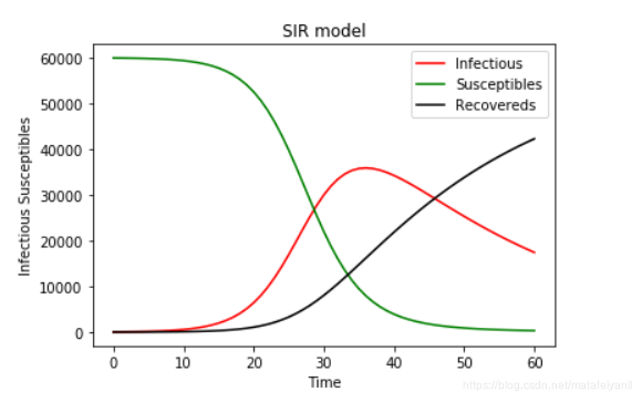
当然，疫情的影响因素过于复杂，我们无法给出精确的预测，只等那春风吹绿东湖的波澜，武大的樱花开满珞珈山，南山之剑斩落病魔。武汉加油！中国加油！