高级编程技术 matplotlib课后作业

Exercise 11.1: Plotting a function

import numpy as np  
import matplotlib.pyplot as plt  
  
x = np.linspace(0, 2, 200)  
f1 = x-2  
f2 = np.exp(-1*np.power(x, 2))  
f3 = np.sin(f1*f2)  
y = np.power(f3, 2)  
  
plt.plot(x, y, 'r', linewidth = 2)  
plt.axis([0, 2, -2, 2])  
plt.text(0.3, 1.3, r'$sin^2{(x-2)*[exp(-x^2)]}$')  
plt.title('11.1', fontsize = 12)  
  
plt.show()  

结果：

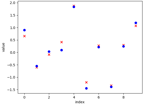
Exercise 11.2: Data

import numpy as np  
import matplotlib.pyplot as plt  
  
X = np.mat(np.random.randn(20, 10))  
b1 = np.mat(np.random.randn(10, 1))  
z = np.mat(np.random.normal(size=(20, 1)))  
y = X*b1+z  
  
x = np.linspace(0, 9, 10)  
b1 = np.array(b1)  
b2 = np.array(np.linalg.lstsq(X, y, rcond = -1)[0])  
plt.scatter(x, b1, c = 'r', marker = 'x', label = "True coefficients")  
plt.scatter(x, b2, c = 'b', marker = 'o', label = "Estimated coefficients")  
plt.xlabel("index")  
plt.ylabel("value")  
plt.title('11.2', fontsize=12)  
plt.show()

结果：

Exercise 11.3: Histogram and density estimation

import numpy as np  
import matplotlib.pyplot as plt  
from scipy import statsz = np.random.normal(size = 10000)

k = stats.gaussian_kde(z)
x = np.linspace(-5, 5, 200)
plt.hist(z, 25, density = True)
plt.plot(x, k.evaluate(x), 'r')
plt.title('11.3', fontsize = 12)
plt.show() 

结果：