吴恩达机器学习ex1

1-单变量线性回归

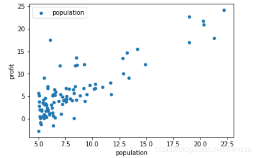
案例：假设你是一家餐厅的CEO，正在考虑开一家分店，根据该城市的人口数据预测其利润。

我们拥有不同城市对应的人口数据以及利润： ex1data1.txt

1. 先引入库

import numpy as np
import pandas as pd
import matplotlib.pyplot as plt

2. 读取数据

data = pd.read_csv('ex1data1.txt',names=['population','profit'])
data.head() #打印前5行看看
---------------------------------------
population	profit
0	6.1101	17.5920
1	5.5277	9.1302
2	8.5186	13.6620
3	7.0032	11.8540
4	5.8598	6.8233
--------------------------------------

data.plot.scatter('population','profit',label='population') #绘制散点图
plt.show()

3. 处理数据

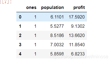
data.insert(0,"ones",1) #为了方便矩阵化运算，先插入一行全为1的值
data.head()

插入完后data长这样

X = data.iloc[:,0:-1] #获取前三列 iloc[行，列]，并且 : 的区间范围左开右闭，比如说这里是[0,-1)
y = data.iloc[:,-1] # 获取最后一列

X = X.values # 将dataframe类型转为数组类型
y = y.values

X.shape #看一下维度
(97, 2)

y.reshape(len(y),1)
y.shape
(97,1)

4. 代价函数

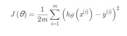
根据公式定义一个代价函数~

def costFunc(X,y,theta):
    inner = np.power((X @ theta)-y,2)
    return np.sum(inner) / (2*len(X))

现在还需要定义下theta

theta = np.zeros((2,1)) #初始化数据为0,
theta.shape
（2,1）


firstCost = costFunc(X,y,theta)
print(firstCost)
32.072733877455676

5. 梯度下降
   为了求得代价函数的最小值，采用梯度下降的方法~
   先定义下梯度下降函数

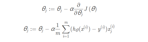
def gradDesc(X,y,theta,alpha,iters): #alpha 学习速率，iters迭代次数
    costs = [] # 记录每次的cost
    for i in range(iters):
        theta = theta - (alpha/len(X) * X.T @ (X@theta -y) )
        cost = costFunc(X,y,theta)
        costs.append(cost)
        
        if(i % 100 == 0):
            print(cost)
    return theta,costs


alpha = 0.02
iters = 1000
theta , costs = gradDesc(X,y,theta,alpha,iters)
print(costs)

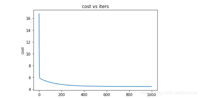
打印costs，看得出代价每次都在减小
16.769642371667462
5.170668092303259
4.813840215803055
4.640559602034057
4.556412109403549
4.5155489085988645
4.495705166048674
4.486068766778817
4.481389196347322
4.479116731414093

通过画图更直观的看一下

fig,ax = plt.subplots()
ax.plot(np.arange(iters),costs)
ax.set(xlabel='iters',
      ylabel='cost',
      title='cost vs iters')
plt.show()

最后，划出拟合的直线

x = np.linspace(y.min(),y.max(),100) #从最小值到最大值的100个均匀的点
y_ = theta[0,0] + x #拟合的直线

fig,ax = plt.subplots()
ax.scatter(X[:,1],y,label='training data')
ax.plot(x,y_,'r',label = 'predict')
ax.legend()
ax.set(xlabel='populaiton',
      ylabel='profit',)
plt.show()