Python与自然语言处理（三）：Tensorflow基础学习

最新推荐文章于 2023-06-18 22:50:38 发布

monkey131499

最新推荐文章于 2023-06-18 22:50:38 发布

阅读量7.9k

点赞数 1

分类专栏： NLP 文章标签： Python tensorflow 神经网络

本文链接：https://blog.csdn.net/monkey131499/article/details/52145254

版权

NLP 专栏收录该内容

20 篇文章 0 订阅

订阅专栏

看了一段时间的TensorFlow，然而一直没有思路，偶然看到一个讲解TensorFlow的系列视频，通俗易懂，学到了不少，在此分享一下，也记录下自己的学习过程。

教学视频链接：点这里

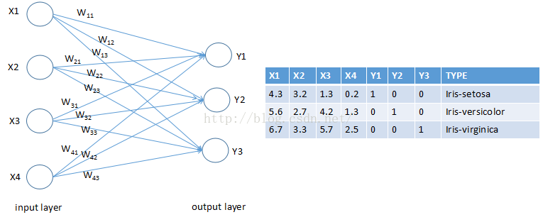
在机器学习中，常见的就是分类问题，邮件分类，电影分类等等

我这里使用iris的数据进行花的种类预测，iris是一个经典的数据集，在weka中也有使用。

iris数据集：点这里

数据集示例：

5.1,3.5,1.4,0.2,Iris-setosa
4.9,3.0,1.4,0.2,Iris-setosa
4.7,3.2,1.3,0.2,Iris-setosa
4.6,3.1,1.5,0.2,Iris-setosa
5.0,3.6,1.4,0.2,Iris-setosa
5.4,3.9,1.7,0.4,Iris-setosa
7.0,3.2,4.7,1.4,Iris-versicolor
6.4,3.2,4.5,1.5,Iris-versicolor
6.9,3.1,4.9,1.5,Iris-versicolor
5.5,2.3,4.0,1.3,Iris-versicolor
6.5,2.8,4.6,1.5,Iris-versicolor
7.1,3.0,5.9,2.1,Iris-virginica
6.3,2.9,5.6,1.8,Iris-virginica
6.5,3.0,5.8,2.2,Iris-virginica
7.6,3.0,6.6,2.1,Iris-virginica

在做分类预测前，我对数据集进行了处理，这里有三种类别的花，分别以（1,0,0）表示Iris-setosa，（0,1,0）表示Iris-versicolor，（0,0,1）表示Iris-virginica

处理后的数据集示例：

4.4,3.2,1.3,0.2,1,0,0
5.0,3.5,1.6,0.6,1,0,0
5.1,3.8,1.9,0.4,1,0,0
5.7,3.0,4.2,1.2,0,1,0
5.7,2.9,4.2,1.3,0,1,0
6.2,2.9,4.3,1.3,0,1,0
5.8,2.7,5.1,1.9,0,0,1
6.8,3.2,5.9,2.3,0,0,1
6.7,3.3,5.7,2.5,0,0,1

思路：

首先，将数据集分成两份，一部分为training set，共120条数据；一部分为testing set，共30条数据。

然后，读取数据文件（txt格式），每条数据的1~4列为输入变量，5~7列为花的种类，所以输入为4元，输出为3元。

之后，初始化权重（weights）和偏量（biase），根据Y=W*X+b进行计算。

最后，计算预测值与真实值的差距，并选择合适的学习速率来减小差距。

具体实现如下：

# -*-coding=utf-*-
import tensorflow as tf
import numpy as np

training_data = np.loadtxt('./MNIST_data/iris_training.txt',delimiter=',',unpack=True,dtype='float32')
test_data = np.loadtxt('./MNIST_data/iris_test.txt',delimiter=',',unpack=True,dtype='float32')

training_data = training_data.T #转置
test_data = test_data.T

#print(training_data.shape)

iris_X = training_data[:,0:4] #[行，列]
iris_Y = training_data[:,4:7]

iris_test_X = test_data[:,0:4]
iris_test_Y = test_data[:,4:7]

def add_layer(inputs,in_size,out_size,activation_function=None):
	Weights = tf.Variable(tf.random_normal([in_size,out_size]))
	biases = tf.Variable(tf.zeros([1,out_size])) + 0.1 #推荐biases最好不为零
	Wx_plus_b = tf.matmul(inputs,Weights) + biases
	if activation_function is None: #activation_function=none表示线性函数，否则是非线性
		outputs = Wx_plus_b
	else:
		outputs = activation_function(Wx_plus_b)
	return outputs

def computer_accuracy(v_xs,v_ys):
	global prediction
	y_pre = sess.run(prediction,feed_dict={xs:v_xs})
	correct_prediction = tf.equal(tf.argmax(y_pre,1),tf.argmax(v_ys,1))
	accuracy = tf.reduce_mean(tf.cast(correct_prediction,tf.float32))
	result = sess.run(accuracy,feed_dict={xs:v_xs,ys:v_ys})
	return result

xs = tf.placeholder(tf.float32,[None,4])
ys = tf.placeholder(tf.float32,[None,3])

prediction = add_layer(xs,4,3,activation_function=tf.nn.softmax) #softmax一般用来做classification

cross_entropy = tf.reduce_mean(-tf.reduce_sum(ys*tf.log(prediction),reduction_indices=[1])) #loss
#学习速率根据 具体使用的数据进行选取
train_step = tf.train.GradientDescentOptimizer(0.001).minimize(cross_entropy)
init = tf.initialize_all_variables()sess = tf.Session()sess.run(init)
for i in range(700): #迭代700次
      sess.run(train_step,feed_dict={xs:iris_X,ys:iris_Y})
      if i % 50 == 0:
            print(computer_accuracy(iris_test_X,iris_test_Y),sess.run(cross_entropy,feed_dict={xs:iris_X,ys:iris_Y})) #测试准确率与训练误差

输出：

第一次测试：
(0.53333336, 1.4005684)
(0.60000002, 1.0901265)
(0.56666666, 0.88059545)
(0.69999999, 0.75857288)
(0.76666665, 0.69699961)
(0.80000001, 0.66695786)
(0.80000001, 0.65065509)
(0.80000001, 0.63982773)
(0.80000001, 0.63119632)
(0.80000001, 0.62356067)
(0.80000001, 0.61648983)
(0.80000001, 0.60982168)
(0.80000001, 0.60348624)
(0.80000001, 0.59744602)

第二次测试：
(0.53333336, 6.5918231)
(0.60000002, 5.4625101)
(0.60000002, 4.4928107)
(0.60000002, 3.6116555)
(0.60000002, 2.8158391)
(0.56666666, 2.094959)
(0.53333336, 1.4308809)
(0.53333336, 0.89007533)
(0.5, 0.61958134)
(0.46666667, 0.53800708)
(0.5, 0.51004487)
(0.46666667, 0.49609584)
(0.5, 0.48745066)
(0.5, 0.48149654)

这里使用的numpy，因此需要对numpy有所了解。这里没有涉及到隐藏层，只有一层输入层和一层输出层，分类的准确率不是太好，每次测试的结果也不相同，应该跟weights的初始值有关；为提高准确率，考虑加入隐藏层，按照这个思路继续尝试！

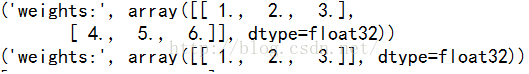
训练生成的网络想要保存下来就需要用到tensorflow.train.Saver()了，下面是一个简单的例子：

import tensorflow as tf
import numpy as np

#save to file
W = tf.Variable([[1.,2.,3.],[4.,5.,6.]],name='weights')
b = tf.Variable([[1.,2.,3.]],name='biases')

init = tf.initialize_all_variables()

saver = tf.train.Saver()

with tf.Session() as sess:
	sess.run(init)
	save_path = saver.save(sess,"./save_net.ckpt") #存储网络到XX路径
	print('Save to path:',save_path)


#restore variables
#redefine the same shape and same type for your variables
<span style="font-size:18px;"></span><pre name="code" class="python">#因为训练时 W和b都是float32的类型，若不指定数据类型会报错

w_type = np.array(np.arange(6).reshape(2,3),dtype=np.float32)b_type = np.array(np.arange(3).reshape(1,3),dtype=np.float32)W = tf.Variable(w_type,name='weights')b = tf.Variable(b_type,name='biases')#not need init stepsaver = tf.train.Saver()with tf.Session() as sess:saver.restore(sess,'./save_net.ckpt') #从XX路径读取网络print('weights:',sess.run(W))print('weights:',sess.run(b))

【output】：