Machine learning : Regression with one variable

学习NG的Machine Learning教程，先关推导及代码。由于在matleb或Octave中需要矩阵或向量，经常搞混淆，因此自己推导，并把向量的形式写出来了，主要包括cost function及gradient descent
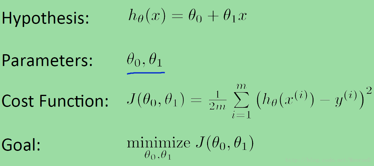
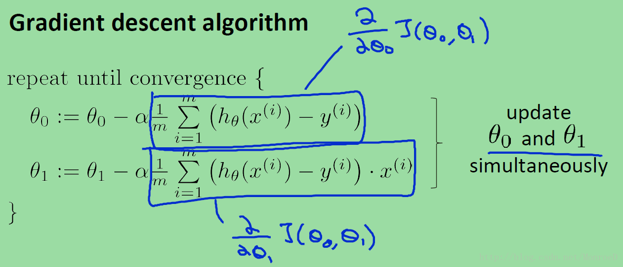
见下图。

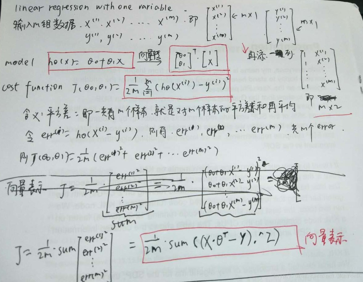
图中可见公式推导，及向量化表达形式的cost function（J）.

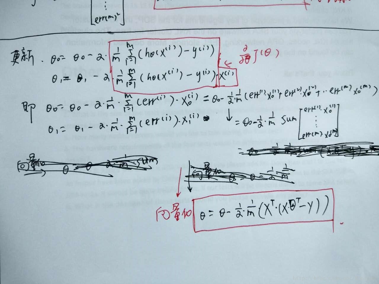
图中为参数更新的向量化表达方式(其中有一处写错了，不想改了。。。)

下面regression with one variable的代码

% regression with one variable
data = load('dat.txt');
X = data(:,1); % X = m*1
y = data(:,2); % y = m*1

% plot data
plot(X,y);

X = [ones(m,1) X]; % X = m*2
theta = zeros(2,1); % theta = 2*1

%gradient descent
iterations = 1500;
alpha = 0.01;

fprintf('\nRunning Gradient Descent ...\n')
theta = gradientDescent(X, y, theta, alpha, iterations);

% print theta to screen
fprintf('Theta found by gradient descent:\n');
fprintf('%f\n', theta);

% Plot the linear fit
hold on; % keep previous plot visible
plot(X(:,2), X*theta, '-')
legend('Training data', 'Linear regression')
hold off % don't overlay any more plots on this figure

其中gradientDescent函数如下

function [theta, J_history] = gradientDescent(X, y, theta, alpha, num_iters)

% Initialize some useful values
m = length(y); % number of training examples
J_history = zeros(num_iters, 1);

%X: m*2 , y:m*1 , theta:2*1, alpha:1*1
for iter = 1:num_iters
    error = (X*theta - y); %m*1
    theta = theta - alpha/m*(X'*(X*theta-y)); 
    J_history(iter) = computeCost(X, y, theta);
end
plot([1:num_iters],J_history); %画图
pause;
end

其中computeCost代码如下

function J = computeCost(X, y, theta)

m = length(y); % number of training examples
J = 0;
error = X * theta - y; % m*1
J = 1/(2*m)*sum(error .^ 2);

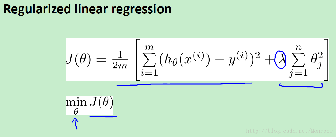
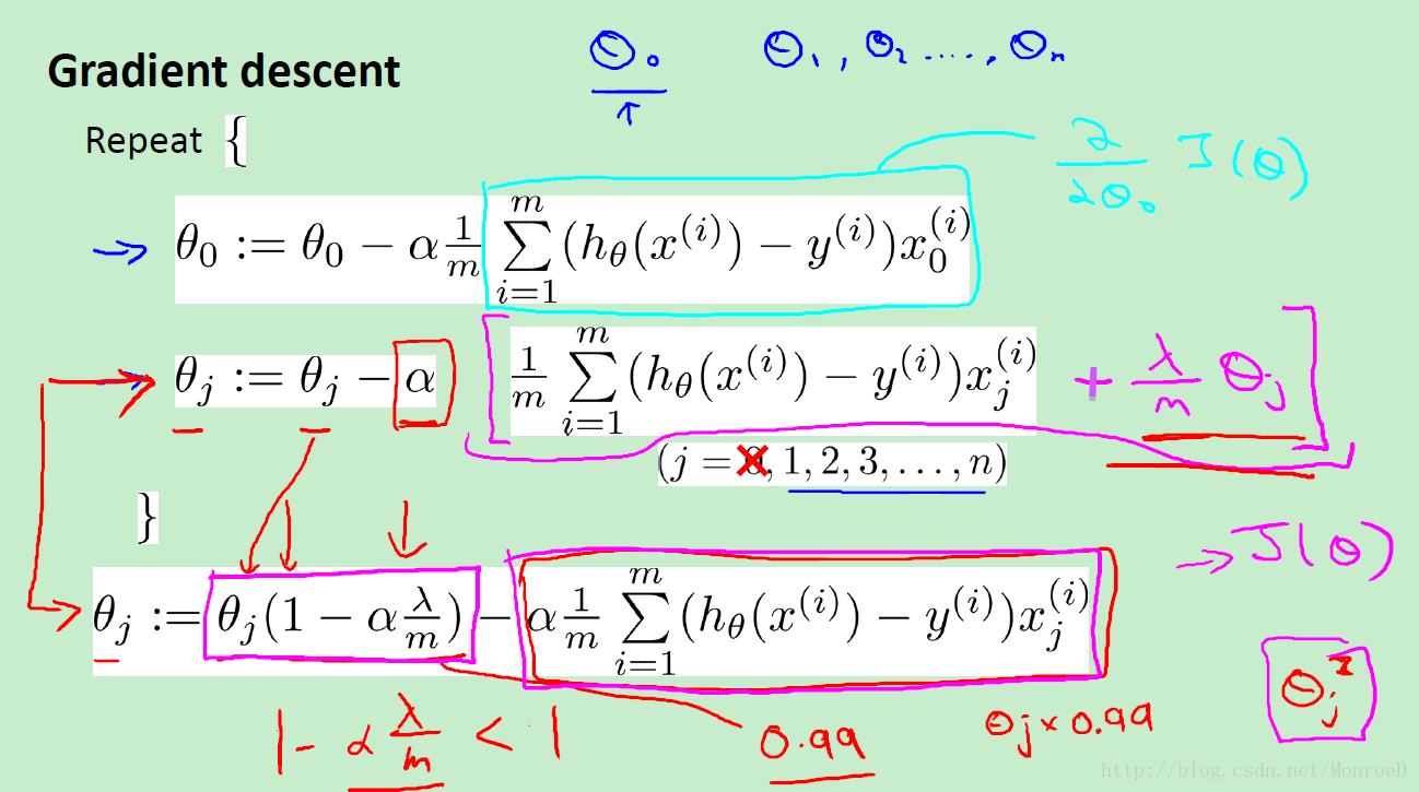
end

下见linear regression 正则化的公式

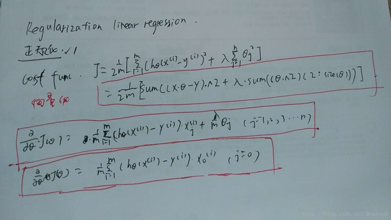
为方便查找，下附公式原图，

以下为regularized linear regression