【知识点】np.random.randn()

目录

一、基本知识

1. np.random.randn()

2. 正态分布

二、具体实例

三、项目应用

---

一、基本知识

1. np.random.randn()

numpy.random.randn(d0,d1,…,dn)

(1) randn函数返回一个或一组样本，具有标准正态分布。

(2) dn表格每个维度

(3) 返回值为指定维度的array

2. 正态分布

标准正态分布介绍

（1）标准正态分布—-standard normal distribution

（2）标准正态分布又称为u分布，是以0为均值、以1为标准差的正态分布，记为N（0，1）。

---

二、具体实例

代码：

import numpy as np

x = np.random.randn(2, 4)
b = np.random.randn(3, 2, 4)
print(f'x is {x}')
print()
print(f'b is {b}')

结果：

x is [[ 0.91998142  1.35255229  0.61680609 -0.90104357]
 [-1.1394227   0.16248028  1.31023715 -0.35412562]]

b is [[[-0.9556731  -0.99616581 -0.19022034 -0.83921712]
  [-0.98856744 -0.77866624 -0.36667162 -1.69963599]]

 [[-1.31725326 -0.22468372 -1.93575552  0.28267799]
  [-0.75844531  0.42178096 -0.63655538 -1.88670984]]

 [[ 0.09319706 -0.36167653 -0.74885749 -0.60621931]
  [-1.05559154  0.09121703 -0.85993236 -0.20603581]]]

---

三、项目应用

代码：

import numpy as np
import matplotlib.pyplot as plt


def sigmoid(x):
    return 1 / (1 + np.exp(-x))


def ReLU(x):
    return np.maximum(0, x)


def tanh(x):
    return np.tanh(x)
    
input_data = np.random.randn(1000, 100)  # 1000个数据
node_num = 100  # 各隐藏层的节点（神经元）数
hidden_layer_size = 5  # 隐藏层有5层
activations = {}  # 激活值的结果保存在这里

x = input_data

for i in range(hidden_layer_size):
    if i != 0:
        x = activations[i-1]  
        #当i=0时，activations是空的，所以不执行该语句
        #当i=1时，activations有上一轮输出的z，此时让x=上一轮的z

    # 改变初始值进行实验！
    w = np.random.randn(node_num, node_num) * 1
    # w = np.random.randn(node_num, node_num) * 0.01
    # w = np.random.randn(node_num, node_num) * np.sqrt(1.0 / node_num)
    # w = np.random.randn(node_num, node_num) * np.sqrt(2.0 / node_num)


    a = np.dot(x, w)


    # 将激活函数的种类也改变，来进行实验！
    z = sigmoid(a)
    # z = ReLU(a)
    # z = tanh(a)

    activations[i] = z

# 绘制直方图
for i, a in activations.items():
    plt.subplot(1, len(activations), i+1)
    plt.title(str(i+1) + "-layer")
    if i != 0: plt.yticks([], [])
    # plt.xlim(0.1, 1)
    # plt.ylim(0, 7000)
    plt.hist(a.flatten(), 30, range=(0,1))
plt.show()

主要看这部分：

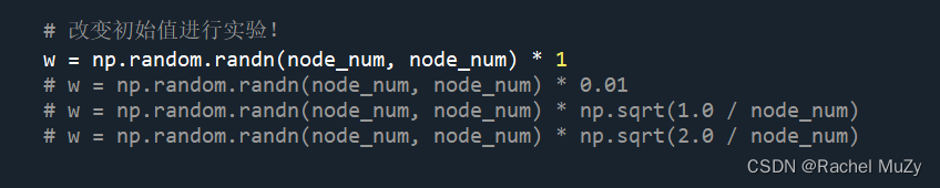（1）*1表示标准差为1的高斯函数

（2）*0.01表示标准差为0.01的高斯函数