基于Python实现的神经网络分类MNIST数据集

神经网络分类MNIST数据集
目录
神经网络分类MNIST数据集 1
一 、问题背景 1
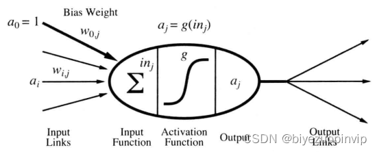
1.1 神经网络简介 1
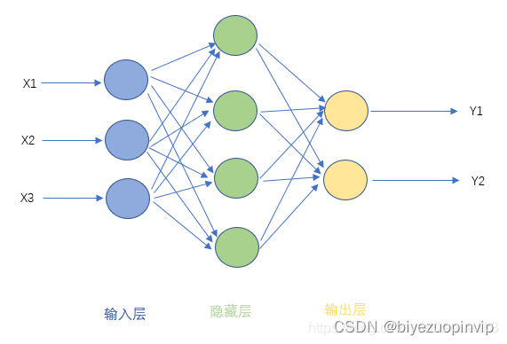
前馈神经网络模型： 1
1.2 MINST 数据说明 4
1.3 TensorFlow基本概念 5
二 、实现说明 5
2.1 构建神经网络模型 5

1. 为输入输出分配占位符 5
2. 搭建分层的神经网络 6
3. 处理预测结果 8
   2.2 运行模型 9
   三 、程序测试 9
   3.1 运行说明 10
   3.2 运行输出 10
   四 、实验总结 11
   2.2运行模型
   首先调用 tf.global_variables_initializer() 初始化模型的参数，Session提供了Operation执行和Tensor求值的环境
   其中：
   模型训练分批次，每一批用100个样本训练神经网络模型，每一批都在上一批的基础上对网络模型 的参数进行调整。
   mnist.train.next_batch ：返回的是一组元组，元组的第一个元素图片像素阵列，第二个元素为 one-hot 格式的预测标签。
   ：在一个Session 里面计算张量的值，执行定义的所有必要的操作来产生这个计算这个张量需要的输入，然后通过这些输入产生这个张量。
   feed_dict 作用是给使用 placeholder 创建出来的张量赋值，上述我们使用 定义
   的占位符包括输入 x 、输出 y 和Dropout 层保留比例 keep_prob 。
   三 、程序测试
   3.1运行说明
   因为实验代码所需要的TensorFlow版本为1.4.0，而现在TensorFlow的版本已经上升到了2.x，一些以前
   提供的数据集、函数已经被删除，故直接运行会报错，报错内容为找不到 包。
   我们可以使用一些Online运行环境，如 Google Colab （https://colab.research.google.com/）。使用云计算来运行我们的程序，将TensorFlow降级至1.4.0，而不修改本地 Python 的配置。
   将TensorFlow降级的方法如下：在文件首行加入以下代码，然后再 import tensorflow 。
   执行程序后会首先出现以下输出，本文转载自http://www.biyezuopin.vip/onews.asp?id=16721程序其他部分无需修改即可以正常运行，运行结果与预期一致。
   3.2运行输出
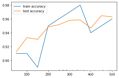
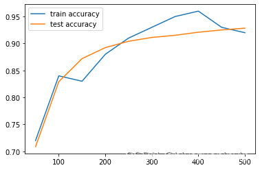
   运行输出如下：可以看到随着测试规模的增加，训练和测试的准确率也不断地在上升。
   step 0, training accuracy 0.07, test accuracy 0.1024
   step 50, training accuracy 0.91, test accuracy 0.8892
   3 step 100, training accuracy 0.95, test accuracy 0.9325
   4 step 150, training accuracy 0.94, test accuracy 0.9405
   5 step 200, training accuracy 0.95, test accuracy 0.9468
   6 step 250, training accuracy 0.96, test accuracy 0.9518
   7 step 300, training accuracy 0.94, test accuracy 0.9543
   8 step 350, training accuracy 0.97, test accuracy 0.9645
   9 step 400, training accuracy 0.94, test accuracy 0.9588
   10 step 450, training accuracy 0.95, test accuracy 0.9655
   11
   12 step 500, training accuracy 1, test accuracy 0.9608
   test accuracy 0.9586
   尝试修改部分参数，观察输出变化情况。
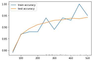
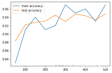
   提高Adam下降算法的学习率：将学习率从 提高到 、
   可以看到随着学习率的提高，测试正确率有明显的提高，但耗时随之上升。
   step 0, training accuracy 0.08, test accuracy 0.1123
   step 50, training accuracy 0.94, test accuracy 0.913
   step 100, training accuracy 0.9, test accuracy 0.9283
   4 step 150, training accuracy 0.95, test accuracy 0.9442
   5 step 200, training accuracy 0.91, test accuracy 0.9413
   6 step 250, training accuracy 0.94, test accuracy 0.954
   7 step 300, training accuracy 0.93, test accuracy 0.9513
   8 step 350, training accuracy 0.99, test accuracy 0.9598
   9 step 400, training accuracy 0.97, test accuracy 0.9609
   10 step 450, training accuracy 0.94, test accuracy 0.9584
   11 step 500, training accuracy 0.96, test accuracy 0.9609
   12 test accuracy 0.9651

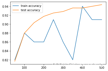
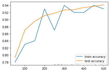
当学习率提高到 时，过高的学习率容易跳过最优值，预测效果反而下降。
step 0, training accuracy 0.07, test accuracy 0.0877
step 50, training accuracy 0.89, test accuracy 0.9095
3 step 100, training accuracy 0.94, test accuracy 0.9233
4 step 150, training accuracy 0.91, test accuracy 0.9267
5 step 200, training accuracy 0.89, test accuracy 0.882
6 step 250, training accuracy 0.96, test accuracy 0.9383
7 step 300, training accuracy 0.92, test accuracy 0.9426
8 step 350, training accuracy 0.96, test accuracy 0.9384
9 step 400, training accuracy 0.95, test accuracy 0.9524
10 step 450, training accuracy 0.93, test accuracy 0.9504
11 step 500, training accuracy 0.95, test accuracy 0.9563
12 test accuracy 0.9469
增加/减少神经网络隐层
经测试，网络层数（3，4，5）对模型效果的影响不明显。而层次相同的神经网络中节点数目多的 表现出性能更优。
四 、实验总结
通过本次实验，我们深入理解了前馈神经网络模型，通过示例代码，研究MINST数据集训练神经网络的过程。第一次了解 TensorFlow，学习了TensorFlow的基本概念和用法，掌握了如何运用
TensorFlow来构建一个神经网络模型。

% tensorflow_version
1.4
.0
import tensorflow as tf
import matplotlib.pyplot as plt
import time

print(tf.__version__)

from tensorflow.examples.tutorials.mnist import input_data

# 加载MNIST数据集，通过设置 one_hot=True 来使用独热编码标签
# 独热编码：对于每个图片的标签 y，10 位中仅有一位的值为 1，其余的为 0。
mnist = input_data.read_data_sets('MNIST_data', one_hot=True)


# 权重正态分布初始化函数
def weight_variable(shape):
    # 生成截断正态分布随机数,shape表示生成张量的维度，mean是均值(默认=0.0)，stddev是标准差。
    # 取值范围为 [ mean - 2 * stddev, mean + 2 * stddev ]，这里为[-0.2, 0.2]
    initial = tf.truncated_normal(shape, stddev=0.1)
    return tf.Variable(initial)


# 偏置量初始化函数
def bias_variable(shape):
    initial = tf.constant(0.1, shape=shape)  # value=0.1, shape是张量的维度
    return tf.Variable(initial)


if __name__ == "__main__":

    # 为训练数据集的输入 x 和标签 y 创建占位符
    x = tf.placeholder(tf.float32, [None, 784])  # None用以指代batch的大小，意即输入图片的数量不定，一张图28*28=784
    y = tf.placeholder(tf.float32, [None, 10])
    # 意思是每个元素被保留的概率，keep_prob=1即所有元素全部保留。大量数据训练时，为了防止过拟合，添加Dropout层，设置一个0~1之间的小数
    keep_prob = tf.placeholder(tf.float32)

    # 创建神经网络第1层，输入层，激活函数为relu
    W_layer1 = weight_variable([784, 500])
    b_layer1 = bias_variable([500])
    h1 = tf.add(tf.matmul(x, W_layer1), b_layer1)  # W * x + b
    h1 = tf.nn.relu(h1)
    # 创建神经网络第2层，隐藏层，激活函数为relu
    W_layer2 = weight_variable([500, 1000])
    b_layer2 = bias_variable([1000])
    h2 = tf.add(tf.matmul(h1, W_layer2), b_layer2)  # W * h1 + b，h1为第1层的输出
    h2 = tf.nn.relu(h2)
    # 创建神经网络第3层，隐藏层，激活函数为relu
    W_layer3 = weight_variable([1000, 300])
    b_layer3 = bias_variable([300])
    h3 = tf.add(tf.matmul(h2, W_layer3), b_layer3)  # W * h2 + b，h2为第2层的输出
    h3 = tf.nn.relu(h3)
    # 创建神经网络第4层，输出层，激活函数为softmax
    W_layer4 = weight_variable([300, 10])
    b_layer4 = bias_variable([10])
    predict = tf.add(tf.matmul(h3, W_layer4), b_layer4)  # W * h3 + b，h3为第3层的输出
    y_conv = tf.nn.softmax(tf.matmul(h3, W_layer4) + b_layer4)
    # 计算交叉熵代价函数
    cross_entropy = tf.reduce_mean(tf.nn.softmax_cross_entropy_with_logits(logits=predict, labels=y))
    # 使用Adam下降算法优化交叉熵代价函数
    train_step = tf.train.AdamOptimizer(1e-4).minimize(cross_entropy)
    # 预测是否准确的结果存放在一个布尔型的列表中
    correct_prediction = tf.equal(tf.argmax(y_conv, 1), tf.argmax(y, 1))  # argmax返回的矩阵行中的最大值的索引号
    # 求预测准确率
    accuracy = tf.reduce_mean(tf.cast(correct_prediction, 'float'))  # cast将布尔型的数据转换成float型的数据；reduce_mean求平均值

    # 初始化
    init_op = tf.global_variables_initializer()

    time_start = time.time()
    i_list = []
    train_acc_list = []
    test_acc_list = []

    with tf.Session() as sess:
        sess.run(init_op)
        for i in range(550):  # 训练样本为55000，分成550批，每批为100个样本
            batch = mnist.train.next_batch(100)
            if i % 50 == 0:  # 每过50批，显示其在训练集上的准确率和在测试集上的准确率
                train_accuracy = accuracy.eval(feed_dict={x: batch[0], y: batch[1], keep_prob: 1.0})
                test_accuracy = accuracy.eval(feed_dict={x: mnist.test.images, y: mnist.test.labels})
                print('step %d, training accuracy %g, test accuracy %g' % (i, train_accuracy, test_accuracy))

                if i != 0:
                    i_list.append(i)
                    train_acc_list.append(train_accuracy)
                    test_acc_list.append(test_accuracy)

            # 每一步迭代，都会加载100个训练样本，然后执行一次train_step，并通过feed_dict，用训练数据替代x和y张量占位符。
            sess.run(train_step, feed_dict={x: batch[0], y: batch[1], keep_prob: 0.5})
        # 显示最终在测试集上的准确率
        print(
            'test accuracy %g' % accuracy.eval(feed_dict={x: mnist.test.images, y: mnist.test.labels, keep_prob: 1.0}))

    time_end = time.time()

    plt.plot(i_list, train_acc_list, label="train accuracy")
    plt.plot(i_list, test_acc_list, label="test accuracy")
    plt.legend()
    plt.show()

    print('Totally cost is', time_end - time_start, "s")