统计机器学习方法 for NLP：基于LDA的主题模型

nghuyong

于 2022-06-25 17:54:25 发布

阅读量362

点赞数

本文链接：https://blog.csdn.net/nghuyong/article/details/127959369

版权

前言

最近在重刷李航老师的《统计机器学习方法》尝试将其与NLP结合，通过具体的NLP应用场景，强化对书中公式的理解，最终形成「统计机器学习方法 for NLP」的系列。这篇将介绍隐含狄利克雷分布，即LDA，并基于LDA完成对论文主题提取的任务。

隐含狄利克雷分布是什么？

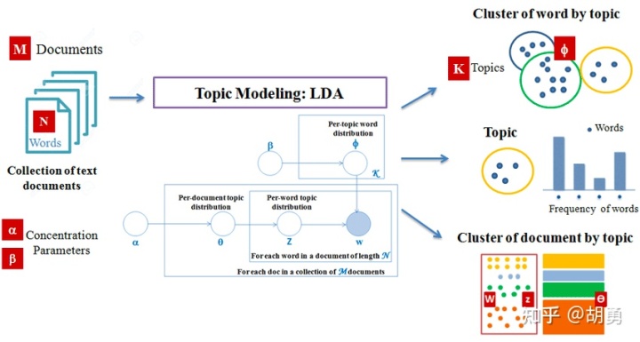
隐含狄利克雷分布(Latent Dirichlet Allocation, LDA) 由戴维·布雷(David Blei)、吴恩达（对，就是那个吴恩达）和迈克尔·乔丹（Michael Jordan）于2003年提出，用来推测文档的主题分布，是一个无监督的生成模型。

首先我们认为每个文档是不同主题的集合，同时每个主题是不同单词的集合。

假定现在整个语料

$D$ 共有

$M$ 篇文档，每篇文档由

$N_{d}$ 个单词构成，一共有

$K$ 个主题。具体生成的步骤如下：

从狄利克雷分布(Dirichlet distribution)
$\alpha$ 中，生成文档

$d$ 的主题分布

$\theta_{d}$
从主题分布
$\theta_{d}$ 中生成文档

$d$ 中第

$n$ 个单词的主题

$z_{d,n}$
从狄利克雷分布(Dirichlet distribution)
$\beta$ 中，生成主题

$z_{d,n}$ 的单词分布

$\phi_{d,n}$
从单词分布
$\phi_{d,n}$ 中生成最终的单词

$w_{d,n}$

所以对于LDA模型，输入

$M$ 篇文档，

$N$ 个单词组成的词表，

$K$ 个主题，模型将输入每个文档的主题分布以及每个主题的单词分布。

对于LDA算法的求解过程为Gibbs采样法，本文先略过，具体可以参考：文本主题模型之LDA(二) LDA求解之Gibbs采样算法。

基于LDA的主题模型

下面我们将基于LDA实现一个对发表在NeurIPS上的2000篇论文，做主题模型的分析。

首先进行数据的加载和数据清洗，只保留论文的正问部分，并且移除文本中的标点符号，停用词，并统一转换成小写，转换完成的数据如下所示：

# data_words
[
    ['actor', 'critic', 'algorithms', 'risk', 'sensitive', 'mdps', 'prashanth', 'la', 'inria', 'lille', ...], 
    ['mixed', 'vine', 'copulas', 'joint', 'models', 'spike', 'counts', 'local', 'field', 'potentials', ...], 
    ['estimating', 'bayes', 'risk', 'sample', 'data', 'robert', 'snapp', 'tong', 'xu', 'computer', ...],
    ...
]

接着我们引入一个词表，并通过基础的词袋模型将文章进行表示

import gensim.corpora as corpora

# Create Dictionary
id2word = corpora.Dictionary(data_words)

# Create Corpus
texts = data_words

# Term Document Frequency
corpus = [id2word.doc2bow(text) for text in texts]

# take a look
print(corpus[0][:30])
"""
[(token_id, token_count),]
[(0, 1), (1, 1), (2, 8), (3, 5), (4, 1), (5, 12), (6, 4), (7, 31), (8, 1), (9, 1), (10, 1), (11, 1), (12, 1), (13, 1), (14, 2), (15, 1), (16, 4), (17, 2), (18, 1), (19, 1), (20, 2), (21, 3), (22, 2), (23, 17), (24, 54), (25, 1), (26, 1), (27, 2), (28, 3), (29, 1)]
"""

下面我们就可以进行LDA模型的训练了，设定有10个类别，这里直接使用gensim.models.LdaMulticore

import gensim

# number of topics
num_topics = 10

# Build LDA model
lda_model = gensim.models.LdaMulticore(corpus=corpus,
                                       id2word=id2word,
                                       num_topics=num_topics)

将10个类别打印出来看一下

pprint(lda_model.print_topics())
[(0,
  '0.006*"data" + 0.006*"model" + 0.005*"learning" + 0.005*"using" + '
  '0.004*"set" + 0.004*"algorithm" + 0.004*"one" + 0.004*"figure" + '
  '0.003*"two" + 0.003*"training"'),
 (1,
  '0.006*"data" + 0.006*"learning" + 0.005*"set" + 0.005*"algorithm" + '
  '0.005*"function" + 0.004*"model" + 0.004*"time" + 0.004*"problem" + '
  '0.003*"using" + 0.003*"matrix"'),
 (2,
  '0.007*"learning" + 0.006*"model" + 0.005*"data" + 0.005*"algorithm" + '
  '0.004*"time" + 0.004*"function" + 0.004*"using" + 0.004*"two" + 0.004*"one" '
  '+ 0.003*"number"'),
 (3,
  '0.007*"learning" + 0.007*"model" + 0.006*"algorithm" + 0.004*"one" + '
  '0.004*"data" + 0.004*"set" + 0.004*"using" + 0.004*"two" + 0.003*"function" '
  '+ 0.003*"results"'),
 (4,
  '0.007*"model" + 0.006*"set" + 0.005*"learning" + 0.005*"data" + '
  '0.004*"using" + 0.004*"algorithm" + 0.004*"function" + 0.004*"models" + '
  '0.003*"time" + 0.003*"training"'),
 (5,
  '0.006*"learning" + 0.006*"algorithm" + 0.005*"data" + 0.005*"one" + '
  '0.004*"model" + 0.004*"set" + 0.004*"function" + 0.004*"using" + '
  '0.004*"number" + 0.003*"time"'),
 (6,
  '0.006*"model" + 0.006*"function" + 0.006*"data" + 0.006*"algorithm" + '
  '0.005*"learning" + 0.005*"set" + 0.004*"using" + 0.004*"two" + 0.003*"one" '
  '+ 0.003*"number"'),
 (7,
  '0.007*"model" + 0.006*"data" + 0.006*"learning" + 0.006*"algorithm" + '
  '0.004*"models" + 0.004*"set" + 0.004*"function" + 0.004*"one" + '
  '0.004*"using" + 0.003*"time"'),
 (8,
  '0.007*"learning" + 0.006*"model" + 0.005*"data" + 0.004*"algorithm" + '
  '0.004*"using" + 0.004*"set" + 0.004*"used" + 0.003*"time" + 0.003*"one" + '
  '0.003*"neural"'),
 (9,
  '0.006*"model" + 0.005*"data" + 0.005*"set" + 0.005*"algorithm" + '
  '0.005*"learning" + 0.004*"function" + 0.004*"using" + 0.004*"problem" + '
  '0.004*"time" + 0.003*"figure"')]

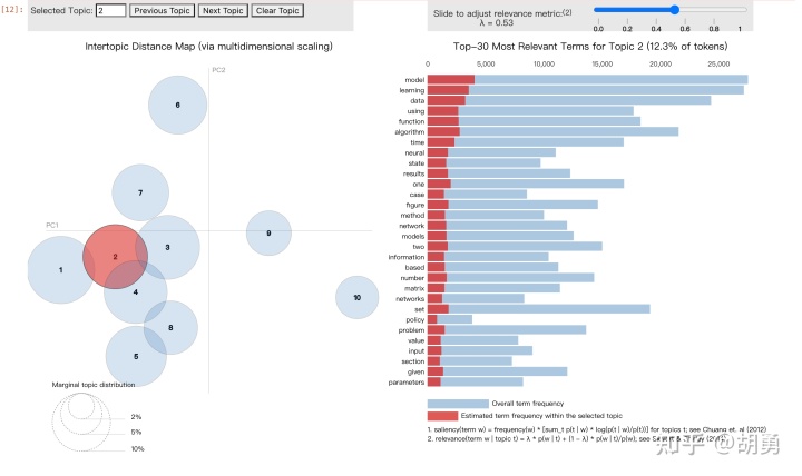
更进一步我们可以采用pyldavis进行进一步交互式的分析，更好看出topic自身的特点以及topic之间的关系

import pyLDAvis.gensim_models
import pyLDAvis

# Visualize the topics
pyLDAvis.enable_notebook()

LDAvis_prepared = pyLDAvis.gensim_models.prepare(lda_model, corpus, id2word)

参考

https://towardsdatascience.com/end-to-end-topic-modeling-in-python-latent-dirichlet-allocation-lda-35ce4ed6b3e0

星环科技：深入机器学习系列11－隐式狄利克雷分布

nghuyong

关注

0
点赞
踩
2

收藏

觉得还不错? 一键收藏
打赏
0
评论
统计机器学习方法 for NLP：基于LDA的主题模型

前言最近在重刷李航老师的《统计机器学习方法》尝试将其与NLP结合，通过具体的NLP应用场景，强化对书中公式的理解，最终形成「统计机器学习方法 for NLP」的系列。这篇将介绍隐含狄利克雷分布，即LDA，并基于LDA完成对论文主题提取的任务。隐含狄利克雷分布是什么？隐含狄利克雷分布(Latent Dirichlet Allocation, LDA) 由戴维·布雷(David Blei)、吴恩达（对...
复制链接

扫一扫