【论文笔记】API-Net：Learning Attentive Pairwise Interaction for Fine-Grained Classification

简介

• 2020年发表在AAAI的一篇细粒度分类论文。
• 人类在区分不同子类的图像时，会成对地进行比较。本文模仿这一行为，同时提取并融合一对图片的特征，提高了网络辨别不同目标的能力。
• 槽点：开源代码环境居然用的 pyton2.7 + torch0.4.1 的远古版本，实验室服务器CUDA10.0完全没法跑😓，以后有机会尝试自己复现吧。。。
• 论文地址
• 代码地址

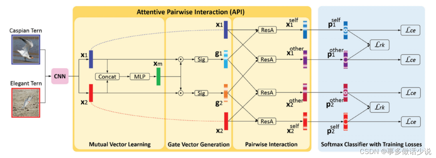
整体框架

创新点

mutual vector learning（互向量学习）

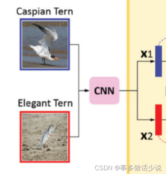
• 训练过程首先把两张图片输入骨干网络 （ResNet101），分别提取D维度的特征 $x_1$ 和 $x_2$，即：$$x_{1}and{x}_2\in {\mathbb{R}}^D$$
  示意图：
  

• 之后进入 互向量学习 阶段，将 $x_1$ 和 $x_2$ 连接，对其使用MLP，即两个全连接加一个Dropout，得到 $x_m\in {\mathbb{R}}^D$。
  $$x_m=f_m([x_1,x_2])，f_m为MLP操作$$

代码：

# 定义
self.map1 = nn.Linear(2048 * 2, 512)
self.map2 = nn.Linear(512, 2048)
self.drop = nn.Dropout(p=0.5)

# concat和两个全连接
mutual_features = torch.cat([features1, features2], dim=1)
map1_out = self.map1(mutual_features)
map2_out = self.drop(map1_out)
map2_out = self.map2(map2_out)

示意图：

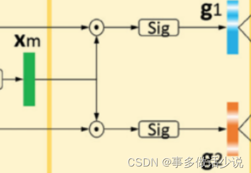
gate vector generation（门向量生成器）

• 先将 x_m 与x₁ 和 x₂ 作比较，从单独的图片中进一步提取有区别的线索（clue），为后续区分这一对做准备。
  • 将 x_m 和x_i 做通道乘积，对结果用sigmoid，生成门函数(gate vector) $g_i\in R^D$

g i = s i g m o i d ( x m ⊙ x i ) , i ∈ { 1 , 2 } g_i=sigmoid(x_m\odot x_i),i\in \left\{1,2 \right\} gi​=sigmoid(xm​⊙xi​),i∈{1,2}

g_i 作为一种区分注意力( discriminative attention)，原文说是通过每个个体 x_i 的不同视角来突出语义差异。其实就是把 x_m 和 x_i 点乘后做 sigmoid，我不认为这一步有多大用🙄。

代码：

gate1 = torch.mul(map2_out, features1) # 点乘
gate1 = self.sigmoid(gate1)

gate2 = torch.mul(map2_out, features2)
gate2 = self.sigmoid(gate2)

示意图：

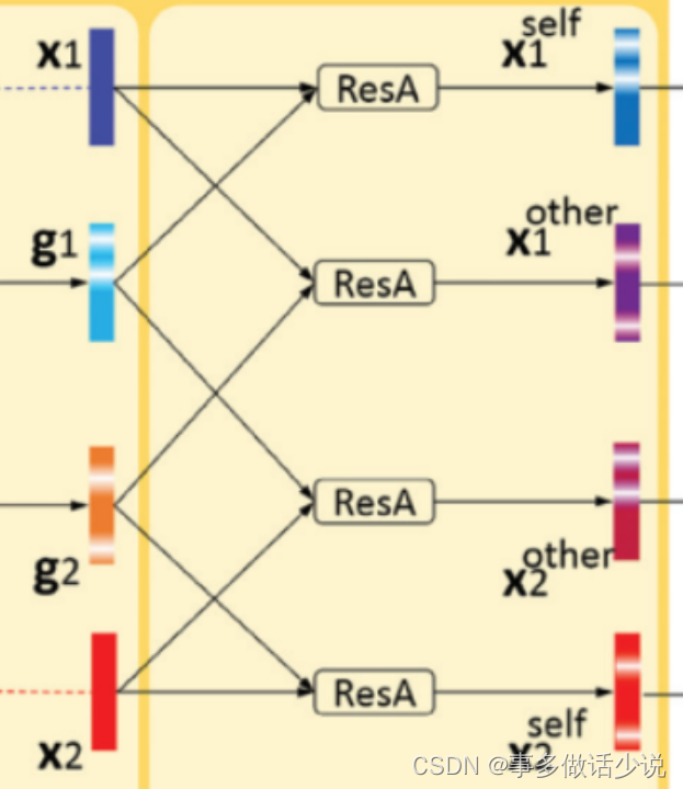
pairwise interaction（成对交互）

• 原文：为了捕捉一对细粒度图像中的细微差异，人类检查每幅图像，不仅有其突出的部分，而且有与其他图像不同的部分。
• 实现：将向量与门两两组合，进行一些操作，得到四个向量：
  • $x_i^{self}$ 用自己的门向量进行加强， $x_i^{other}$ 用自己的门向量和pair中另一副图像进行激活。
  • 用来自这两幅图像的鉴别线索（ discriminative clues）来增强 x_i 。
    $$\begin{gathered} x_1^{self}=x_1+x_1\odot g_1, \\ {x}_2^{self}=x_2+x_2\odot g_2, \\ {x}_1^{other}=x_1+x_1\odot g_2, \\ {x}_2^{other}=x_2+x_2\odot g_1, \end{gathered}$$

代码：

# 点乘后相加
 features1_self = torch.mul(gate1, features1) + features1
 features1_other = torch.mul(gate2, features1) + features1
 features2_self = torch.mul(gate2, features2) + features2
 features2_other = torch.mul(gate1, features2) + features2
 
#全连接后dropout，得到结果
 logit1_self = self.fc(self.drop(features1_self))
 logit1_other = self.fc(self.drop(features1_other))
 logit2_self = self.fc(self.drop(features2_self))
 logit2_other = self.fc(self.drop(features2_other))

示意图：

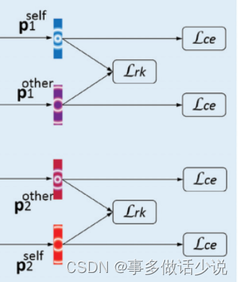
之后便是常规的softmax以及计算损失，得到最终结果。
值得一提的是，计算损失过程中除了交叉熵损失，还添加了一个排序损失 $L_{rk}$ 。
作用是让 $p_i^{other}$ 的优先级更低。
其实就是MarginRankingLoss：

L r k = ∑ i ∈ { 1 , 2 } m a x ( 0 , p i o t h e r ( c i ) − p i s e l f ( c i ) + ξ ) L_{rk}=\sum_{i\in \left \{ 1,2 \right\}}max(0,p^{other}_i(c_i)-p^{self}_i(c_i)+\xi) Lrk​=i∈{1,2}∑​max(0,piother​(ci​)−piself​(ci​)+ξ)

# 定义
criterion = nn.CrossEntropyLoss().to(device)
rank_criterion = nn.MarginRankingLoss(margin=0.05)

# 实现
softmax_loss = criterion(logits, targets)
rank_loss = rank_criterion(self_scores, other_scores, flag)
loss = softmax_loss + rank_loss

示意图：

队构造（Pair Construction）

利用欧氏距离找到每张图像和batch中类间图象以及类内图像最接近的两对
细节如下：

• 在一批（batch）中随机抽取 $N_{cl}$ 个类，在每个类中随机抽取 $N_{im}$ 个训练图像；
• 我们将所有这些图像输入CNN主干，生成它们的特征向量；
• 根据欧氏距离，将每幅图像的特征和batch中其他图像的特征进行比较；
• 对每张图像构造出1）类内/类间pair，包含本身的特征，2）batch中类内/类间最相近的特征组成；
• 所以，每一个batch中有 $2\times N_{cl}\times N_{im}$ 个pair；
• 把它们所有的损失L进行总结并进行端到端训练。

代码：

def get_pairs(self, embeddings, labels): # 得到的结果不影响网络梯度
        distance_matrix = pdist(embeddings).detach().cpu().numpy() # detach()：不计算梯度 转到numpy

        labels = labels.detach().cpu().numpy().reshape(-1,1)# 变成一列
        num = labels.shape[0] # 个数
        dia_inds = np.diag_indices(num) # 得到num维数组的对角线的索引
        lb_eqs = (labels == labels.T)
        lb_eqs[dia_inds] = False
        dist_same = distance_matrix.copy()
        dist_same[lb_eqs == False] = np.inf
        intra_idxs = np.argmin(dist_same, axis=1) # 按行取最小值

        dist_diff = distance_matrix.copy()
        lb_eqs[dia_inds] = True
        dist_diff[lb_eqs == True] = np.inf
        inter_idxs = np.argmin(dist_diff, axis=1)

        intra_pairs = np.zeros([embeddings.shape[0], 2])
        inter_pairs  = np.zeros([embeddings.shape[0], 2])
        intra_labels = np.zeros([embeddings.shape[0], 2])
        inter_labels = np.zeros([embeddings.shape[0], 2])
        for i in range(embeddings.shape[0]):
            intra_labels[i, 0] = labels[i]
            intra_labels[i, 1] = labels[intra_idxs[i]]
            intra_pairs[i, 0] = i
            intra_pairs[i, 1] = intra_idxs[i]

            inter_labels[i, 0] = labels[i]
            inter_labels[i, 1] = labels[inter_idxs[i]]
            inter_pairs[i, 0] = i
            inter_pairs[i, 1] = inter_idxs[i]

        intra_labels = torch.from_numpy(intra_labels).long().to(device)
        intra_pairs = torch.from_numpy(intra_pairs).long().to(device)
        inter_labels = torch.from_numpy(inter_labels).long().to(device)
        inter_pairs = torch.from_numpy(inter_pairs).long().to(device)

        return intra_pairs, inter_pairs, intra_labels, inter_labels

实验结果

CUB-200-2011

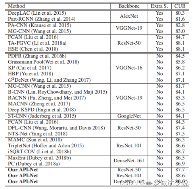
其余不再列举。

总结

• 我个人认为本文的实验结果不算惊艳，网络中的很多步骤我也不明白为啥能够得到正反馈，包括作者自己也只是概括地介绍。
• 但必须承认API-Net的思路很有创新性，并且也能够取得较高的精度。