备战数学建模28 & 科研必备 Python之数据处理神器pandas

目录

1-series和读取外部数据

2-pandas的DataFrame

3-统计方法和字符串离散化

4-数据的合并和分组聚合

---

1-series和读取外部数据

我们知道在python在使用numpy可以处理数值型数据，但是这是远远不够的，因为除了数值数据之外，还有字符串，时间序列等等，所以我们需要使用pandas进行处理；

pandas中常用数据类型：Series一维，带标签的数组；DataFrame二维，Series容器；

python代码如下：

import pandas as pd

t = pd.Series([1,2,31,12,3,4])
print(t)
print(type(t))
print("*" * 100)

#pandas生成一维带标签数组，并设置标签
t2 = pd.Series([1,23,2,2,1], index=list("abcde"))
print(t2)
print("*" * 100)

#pandas通过字典的方式创建Series数组
temp_dict = {"name":"xiaoming", "age":13, "tel":10086}
t3 = pd.Series(temp_dict)
print(t3)
print(t3[0]) #通过索引取值
print(t3["name"]) #通过键取值
print(t3[1:]) #取得连续的行
print(t3[[0,2]]) #取不连续的行
print(t3.index) #找到键
print(len(t3.index))#键的个数
print(t3.values)
print(type(t3.values))
print("*" * 100)

2-pandas的DataFrame

使用pandas读取外部数据，DataFrame和Series，前者二维，后者是一维，前者是后者的容器，我们看一下使用pandas读取文件，以及在pandas中创建DataFrame的过程，具体的代码如下所示：

import pandas as pd
import numpy as np

#pandas直接从当前文件夹下读取文件
p = pd.read_csv("./data/ratings.csv")
#dataFrame对象既有行索引，又有列索引
t = pd.DataFrame(np.arange(12).reshape((3,4)))
print(t)
print("*" * 100)
t1 = pd.DataFrame(np.arange(12).reshape((3,4)), index=list("abc"),columns=list("wxyz"))
print(t1)
print("*" * 100)
#pandas按字典创建dataFrame数组
d = {"name":["xiaoming", "xiaohua"], "age":[17, 18], "tel":[10086, 10010]}
t2 = pd.DataFrame(d)
print(t2)
print("*" * 100)
d2 = [{"name":"xiaoming","age":13,"tel":10086},{"name":"xiaohua","tel":10010},{"name":"xiaohong","age":19}]
t3 = pd.DataFrame(d2)
print(t3)
print("*" * 100)

#行索引
print(t2.index)
#列索引
print(t2.columns)
#值
print(t2.values)
print(t2.shape)#形状
print(t2.dtypes)#每一列的类型
print("*" * 100)
print(t3.head(1)) #显示前1行
print(t3.tail(1)) #显示最后一行
print("*" * 100)
print(t3.info()) #显示相关信息
print("*" * 100)
print(t3.describe()) #显示数字相关信息
print("*" * 100)

对于统计的名字数据，我想知道哪些名字的使用次数比较高，那么使用pandas该怎么实现呢？显然我们需要进行排序处理，另外我们可以使用pandas进行取行和取列操作，具体代码如下：

import pandas as pd
import numpy as np

df = pd.read_csv("./data/dogNames2.csv")
#print(df.head())
#print(df.info())

#DataFrame中的排序方法
df = df.sort_values(by="Count_AnimalName",ascending=False)#降序排序
print(df[:20]) #取前20个
print("*" * 100)
print(df[:20]["Row_Labels"]) #取前20行的Row_Labels列

#df.loc通过标签索引行数据
t3 = pd.DataFrame(np.arange(12).reshape(3,4), index=list("abc"), columns=list("wxyz"))
print(t3)
print(t3.loc["a"]["z"]) #打印a行z列的数据
print(t3.loc[:]["y"]) #取列
print(t3.loc["a"][:]) #取行
print(t3.loc[["a","c"]]) #取多行

#df.iloc通过位置索引行数据
print(t3.iloc[1]) #取行
print(t3.iloc[:,[2,1]]) #取列
print(t3.iloc[1:,2:]) #取固定行列

我们继续学习bool索引和缺失数据的处理，有些时候需要对数据列进行多条件的筛选，那么就需要使用bool索引了，我们直接看代码吧：

import pandas as pd
import numpy as np

df = pd.read_csv("./data/dogNames2.csv")
#print(df.head())
#print(df.info())

df1 = df[(df["Count_AnimalName"] > 800) & (df["Count_AnimalName"] < 1000)] #找到大于800小于1000的
df2 = df[(df["Count_AnimalName"] > 800) | (df["Count_AnimalName"] < 1000)] #大于800或者小于1000的
print(df1)
print("*" * 100)
print(df2)
print("*" * 100)
#找到使用次数超过700且字符串长度大于4的狗的名字
print(df[(df["Count_AnimalName"] > 700) & (df["Row_Labels"].str.len()>4)])
print("*" * 100)

ts = np.arange(24).reshape(4,6).astype(float)
ts[[0,0,3],[0,5,2]] = np.nan

t3 = pd.DataFrame(ts, index=list("abcd"), columns=list("uvwxyz"))

print(t3)
print("*" * 100)
print(pd.isnull(t3)) #t3中的null值
print(pd.notnull(t3)) #t3中的非null值
print("*" * 100)
print(t3.dropna(axis=0,how="all")) #删除当前行全为null的
print(t3.dropna(axis=0,how="any")) #删除当前行存在为null的
print("*" * 100)
print(t3.fillna(100)) #NAN位置填充100
print("*" * 100)
#t3.dropna(axis=0,how="any",inplace=True) #inplace原地修改
#print(t3)
#rint("*" * 100)
print(t3.fillna(t3.mean())) #填充均值
t3[t3==0] = np.nan #认为0为缺失值可以赋值为nan

3-统计方法和字符串离散化

我们现在有2006年到2016年1000部最流行的电影数据，我需要知道这些电影数据中的电影评分的平均分，导演的人数信息，我们该怎么获取呢？我们使用pandas获取电影数据的评分均值，导演人数，演员人数，电影时长的最大值，最小值，均值等等。具体的代码如下所示：

vimport pandas as pd

df = pd.read_csv("./data/IMDB-Movie-Data.csv")
print(df)
print("*" * 100)
print(df.head(1))
print("*" * 100)
#获取评分
print(df["Rating"].mean())
#获取导演的人数
print(len(set(df["Director"].tolist()))) #用set集合去重
print(len(df["Director"].unique())) #用unique去重
print("*" * 100)
#获取演员的人数
temp_actors_list = df["Actors"].str.split(", ").tolist()
actors_list = [i for j in temp_actors_list for i in j]
actors_num = len(set(actors_list))
print(actors_num)
print("*" * 100)
#电影时长的最大值，最小值
max_runtime = df["Runtime (Minutes)"].max()
max_runtime_index = df["Runtime (Minutes)"].argmax()
min_runtime = df["Runtime (Minutes)"].min()
min_runtime_index = df["Runtime (Minutes)"].argmin()
median_runtime = df["Runtime (Minutes)"].median()
print(max_runtime)
print(max_runtime_index)
print(min_runtime)
print(min_runtime_index)
print(median_runtime)

对于一组电影数据，如果我们想知道rating和runtime的情况，应该如何呈现数据呢？具体的过程如下所示：首先绘制运行时间的直方图，代码和绘制结果如下：

import pandas as pd
from matplotlib import pyplot as plt
df = pd.read_csv("./data/IMDB-Movie-Data.csv")

#数据准备
runtime_data = df["Runtime (Minutes)"].values
max_time = runtime_data.max()
min_time = runtime_data.min()

#计算组数
num_bin = (max_time - min_time) // 5


#设置图片大小
plt.figure(figsize=(20,8),dpi=80)
plt.hist(runtime_data,num_bin)
plt.xticks(range(min_time,max_time+5,5))
plt.show()

4-数据的合并和分组聚合

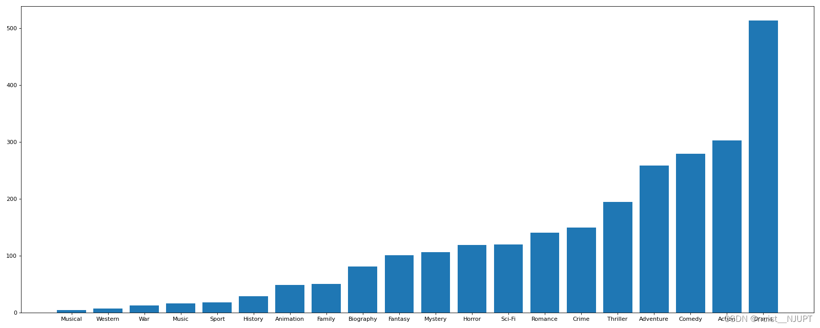
对于一组电影数据，如果我们希望通过电影的分类情况，应该如何处理呢？我们看一下下面的源代码：

import pandas as pd
from matplotlib import pyplot as plt
import numpy as np

df = pd.read_csv("./data/IMDB-Movie-Data.csv")
print(df["Genre"].head(3))
#统计分类的列表
temp_list = df["Genre"].str.split(",").tolist()
gerne_list = list(set([i for j in temp_list for i in j]))

#构造全0的数组
zeros_df = pd.DataFrame(np.zeros((df.shape[0],len(gerne_list))),columns=gerne_list)
#每个电影出现分类的位置赋值1
for i in range(df.shape[0]):
    zeros_df.loc[i,temp_list[i]] = 1
#统计每个分类的电影数量和
gerne_count = zeros_df.sum(axis=0)
print(gerne_count)

#排序
gerne_count = gerne_count.sort_values()
_x = gerne_count.index
_y = gerne_count.values

#画图
plt.figure(figsize=(20,8),dpi=80)
plt.bar(range(len(_x)),_y)
plt.xticks(range(len(_x)),_x)
plt.show()

 下面我们看一下数据合并值join，默认情况下，把行索引相同的合并到一起。还有merge的使用，具体如下代码所示：

import pandas as pd
from matplotlib import pyplot as plt
import numpy as np

df1 = pd.DataFrame(np.ones((2,4)),index=["A","B"],columns=list("abcd"))
print(df1)
print("*" * 100)
df2 = pd.DataFrame(np.zeros((3,3)),index=["A","B","C"],columns=list("xyz"))
print(df2)
print("*" * 100)
print(df1.join(df2))
print("*" * 100)
print(df2.join(df1))
print("*" * 100)

df3 = pd.DataFrame(np.arange(9).reshape(3,3), columns=list("fax"))
print(df3)
print("*" * 100)
print(df1.merge(df3,on="a"))
print("*" * 100)
print(df1.merge(df3,on="a",how="inner"))
print("*" * 100)
print(df1.merge(df3,on="a",how="outer")) #并集
print("*" * 100)

现在我们有一组关于全球星巴克店铺的数据，如果我想知道美国的星巴克数量和中国的哪个多，或者我想知道中国的每个省份的星巴克数量情况，那我该怎么办呢？直接看代码吧：

import pandas as pd
from matplotlib import pyplot as plt
import numpy as np

file_path = "./data/starbucks_store_worldwide.csv"
df = pd.read_csv(file_path)

#调用聚合方法
grouped = df.groupby(by="Country") #按国家分组
coutry_count = grouped["Brand"].count()#按照品牌计数
print(coutry_count["US"])#美国的数量
print(coutry_count["CN"])#中国的数量

#统计中国每个省店铺的数量
china_data = df[df["Country"] == "CN"]
group = china_data.groupby(by="State/Province").count()["Brand"]
print(group)

#按照多个条件进行分组，返回Serier
groups = df["Brand"].groupby(by=[df["Country"],df["State/Province"]]).count()
print(groups) #得到的是带有两个索引的Series类型
print("*" * 100)
#按照多条件进行分组，返回DataFrame
group1 = df[["Brand"]].groupby(by=[df["Country"],df["State/Province"]]).count()
print(group1,type(group1))

下面我们学习一下pandas中的索引和复合索引的相关知识，具体的直接看代码就行，都加了注释的，具体如下：

import pandas as pd
from matplotlib import pyplot as plt
import numpy as np

file_path = "./data/starbucks_store_worldwide.csv"
df = pd.read_csv(file_path)


group1 = df[["Brand"]].groupby(by=[df["Country"],df["State/Province"]]).count()

#索引的方法和属性
print(group1.index)
df1 = pd.DataFrame(np.ones((2,4)),index=["A","B"],columns=list("abcd"))
df1.index = ["a","b"] #给索引赋值
print(df1)
#重新设置index
print(df1.reindex(["a","f"])) #取不到的值为NAN
print(df1.set_index("a",drop=False)) #将DataFrame的某一列作为索引，保留原列

a = pd.DataFrame({'a':range(7),'b' : range(7,0,-1),'c':['one','one','one','two','two','two','two'],'d':list("hjklmno")})
b = a.set_index(["c","d"]) #设置c,d为符合索引
print(b)

d = a.set_index(["d","c"])["a"]
print(d)
print(d.swaplevel()["one"]) #交换内外层索引位置，当想从内层索引取值的时候可以使用swaplevel()方法
print(b.loc["one"].loc["h"]) #根据索引定位
print(b.swaplevel().loc["h"]) #交换内外层索引后的取行操作

我们看一下下面的2个例子：

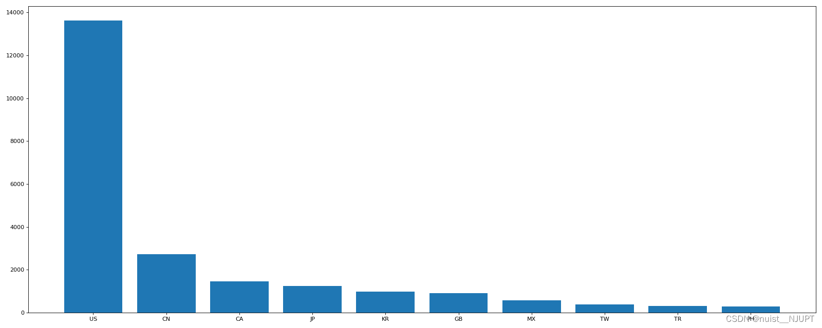
1-使用matplotlib呈现出店铺总数排名前10的国家；

2-使用matplotlib呈现出每个中国每个城市的店铺数量； 

例子1的python代码如下：

import pandas as pd
from matplotlib import pyplot as plt
import numpy as np

file_path = "./data/starbucks_store_worldwide.csv"
df = pd.read_csv(file_path)

data1 = df.groupby(by="Country").count()["Brand"].sort_values(ascending=False)[:10]

_x = data1.index
_y = data1.values

plt.figure(figsize=(20,8),dpi=80)
plt.bar(range(len(_x)),_y)
plt.xticks(range(len(_x)),_x)
plt.show()

绘制的图形如下：

例子2的python代码如下：

 

import pandas as pd
from matplotlib import pyplot as plt
import matplotlib

matplotlib.rc("font", family='YouYuan')

file_path = "./data/starbucks_store_worldwide.csv"
df = pd.read_csv(file_path)
df = df[df["Country"]=="CN"]

data1 = df.groupby(by="City").count()["Brand"].sort_values(ascending=False)[:25] #取前25个城市

_x = data1.index
_y = data1.values

plt.figure(figsize=(20,8),dpi=80)
plt.bar(range(len(_x)),_y,width=0.3,color='orange')
plt.xticks(range(len(_x)),_x)
plt.show()

绘制的图形如下所示：

 绘制横向条形图代码：

import pandas as pd
from matplotlib import pyplot as plt
import matplotlib

matplotlib.rc("font", family='YouYuan')

file_path = "./data/starbucks_store_worldwide.csv"
df = pd.read_csv(file_path)
df = df[df["Country"]=="CN"]

data1 = df.groupby(by="City").count()["Brand"].sort_values(ascending=False)[:25] #取前25个城市

_x = data1.index
_y = data1.values

plt.figure(figsize=(20,8),dpi=80)
plt.barh(range(len(_x)),_y,height=0.3,color='orange')
plt.yticks(range(len(_x)),_x)
plt.show()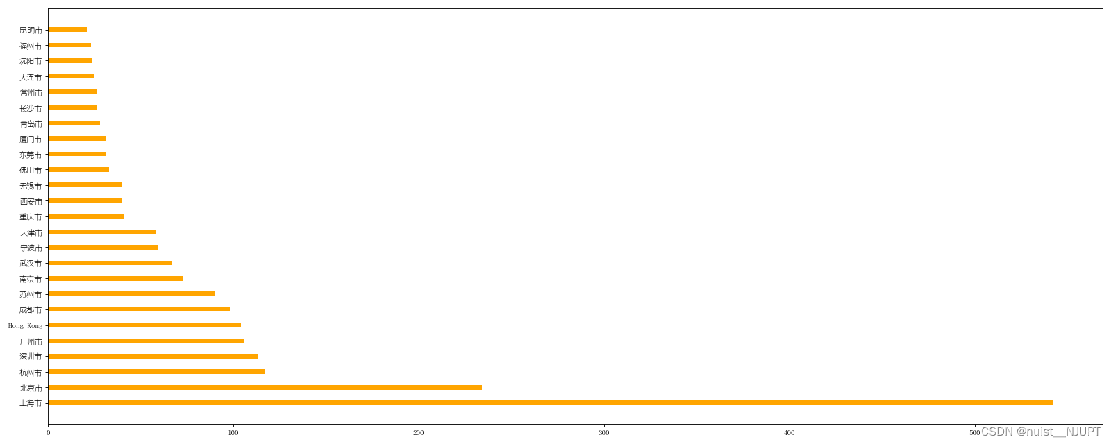

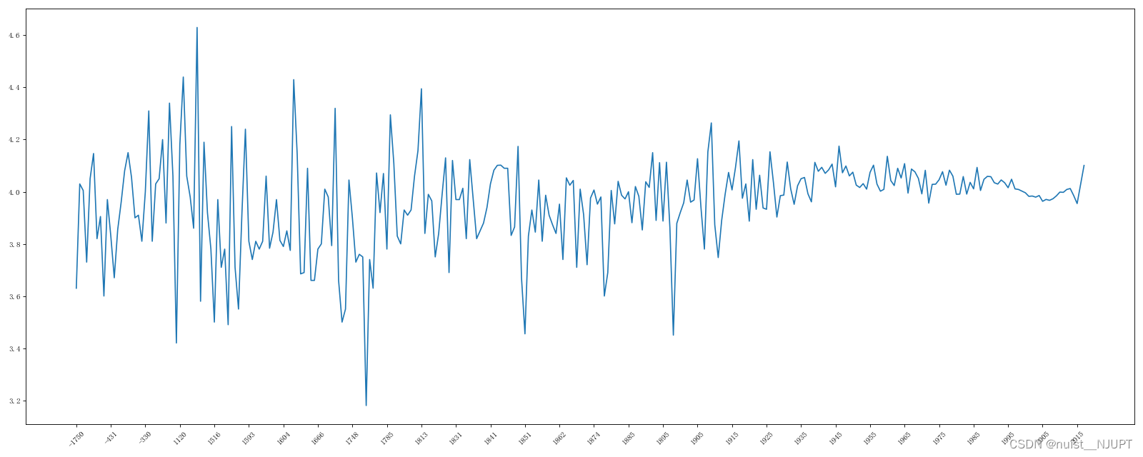
 我们现在有全球排名靠前的10000本书的数据，那么请统计一下下面的几个问题：

1-不同年份书的数量 ；

2-不同年份书的平均评分情况；

上述例子python代码如下：

import pandas as pd
from matplotlib import pyplot as plt
import matplotlib

matplotlib.rc("font", family='YouYuan')

file_path = "./data/books.csv"
df = pd.read_csv(file_path)
data1 = df[pd.notnull(df["original_publication_year"])] #找到非空的年份
group1 = data1.groupby(by="original_publication_year").count()["title"]
print(group1)
print("*" * 100)

#不同年份书的平均评分情况
group2 = data1["average_rating"].groupby(by=data1["original_publication_year"]).mean()
_x = group2.index
_y = group2.values

plt.figure(figsize=(20,8), dpi=80)
plt.plot(range(len(_x)),_y)
plt.xticks(list(range(len(_x)))[::10],_x[::10].astype(int),rotation=45)
plt.show()

绘制的图形如下：