


文章目录
摘要
In terms of papers, I read CNN related papers, which introduced the structure of the AlexNet model and how to solve overfitting; in terms of projects, I summarize some tips when debugging projects; In terms of code, I learn about gradient descent from linear regression and mathematical derivation, and built the simplest neural network to solve multivariate homogeneous equations.
在论文方面,我对CNN相关论文进行了阅读,论文介绍了AlexNet模型的结构,以及解决过拟合的方法;在项目方面,我总结了在调试项目时的一些小技巧;在代码方面,我从线性回归和数学推导去了解梯度下降,搭建了最简单的神经网络实现解多元齐次方程组。
一、文献阅读
1.Title
文章链接:ImageNet Classification with Deep Convolutional Neural Networks
2.Abstract
We trained a large, deep convolutional neural network to classify the 1.2 million high-resolution images in the ImageNet LSVRC-2010 contest into the 1000 different classes. On the test data, we achieved top-1 and top-5 error rates of 37.5% and 17.0% which is considerably better than the previous state-of-the-art. The neural network, which has 60 million parameters and 650,000 neurons, consists of five convolutional layers, some of which are followed by max-pooling layers,and three fully-connected layers with a final 1000-way softmax. To make training faster, we used non-saturating neurons and a very efficient GPU implementation of the convolution operation. To reduce overfitting in the fully-connected layers we employed a recently-developed regularization method called “dropout”that proved to be very effective. We also entered a variant of this model in the ILSVRC-2012 competition and achieved a winning top-5 test error rate of 15.3%,compared to 26.2% achieved by the second-best entry.
我们训练了一个大型的深度卷积神经网络,将ImageNet ILSVRC -2010竞赛中的120万幅高分辨率图像分类为1000个不同的类。在测试数据上,我们的分别top-1和top-5错误率分别为37.5%和17.0%,比之前的水平有了很大的提高。该神经网络有6000万个参数和65万个神经元,由5个卷积层(其中一些是Max pooling池化层)和3个全连接层(最后的1000路softmax层)组成。为了使训练更快,我们使用了非饱和神经元和一个非常高效的GPU卷积运算方式(p.s.使用了Relu和双路GPU)。为了减少全连通层的过拟合,我们采用了一种最近开发的正则化方法“Dropout”,该方法被证明是非常有效的。我们还在ILSVRC-2012比赛中加入了该模型的一个变体,并以top-5测试错误率15.3%获胜,而第二名则是26.2%。
3.论文解读
3.1 Introduction
本文设计并训练了一个5层卷积+3个全连接层的超大卷积神经网络,并使用了当时很多较为先进的模块和技术,使得大模型的训练成为可能,同时一定程度上缓解了大模型的过拟合问题。
3.1.1 ImageNet数据集
ImageNet是一个包含超过1500万张高分辨率图像的数据集,属于大约22000个类别。这些图片是从网上收集来的,并由人工贴标签者使用Amazon的土耳其机器人众包工具进行标记。从2010年开始,作为Pascal Visual Object Challenge的一部分,每年都会举办一场名为ImageNet大型视觉识别挑战赛(ILSVRC)的比赛。ILSVRC使用ImageNet的一个子集,每个类别大约有1000张图片。总共大约有120万张训练图像、5万张验证图像和15万张测试图像。
3.1.2 卷积神经网络(Convolutional Neural Network)
CNN 对于图像的处理,具有一系列的优势:
1)模型容量可以通过模型的深度和宽度来控制。
2)具有强而合理的先验假设。
3)相较于同等层数的全连接网络来说,连接更为稀疏,参数量更少,更容易优化。
3.2 模型结构
3.2.1 ReLU 激活函数
之前对于神经元的输出的建模大多使用的是f(x) = tanh(x)或者是f(x) = (1 + e ^ (-x)) ^ (-1) 这种饱和性非线性函数,而本文改用了一种更为简单的非线性激活函数(ReLUs)。这种激活函数最大的优点在于其前向以及反向传播的计算都很简单,而且不太会出现梯度消失或者爆炸的情况,比较容易训练和收敛。
论文在一个 4 层的卷积神经网络做了实验,对比了使用 ReLU 和 Tanh 两种激活函数的收敛速度:

可以发现在达到同样的正确率的情况下,使用 ReLU 的模型收敛得更快,从而极大地减少了训练所需要的时间。
3.2.2 多GPU并行训练
论文中展示的多GPU并行训练是在当时GPU的内存较小的情况下,采用的无奈操作,得益于现在GPU内存的高速发展,此类操作如今没有使用的必要了。
3.2.3 局部响应归一化(Local Response Normalization)
论文中提出,采用LRN局部响应正则化可以提高模型的泛化能力,所以在某些层应用了ReLU后,加上了LRN使得top-1和top-5的错误率分别降低了1.4%和1.2%。
3.2.4 重叠池化(Overlapping Pooling)
AlexNet 强调了重叠池化的作用,重叠池化实际上就是池化的 kernel size 大于 stride 的情况。
3.2.5 整体结构

上图是AlexNet的整体结构图,就模型设计而言,整体是遵循卷积层提特征降维,全连接层完成分类任务的范式。
不同的设计:
1)在第二、第四和第五个卷积层使用的是分组卷积。
2)在第一个和第二个卷积后使用了 LRN。
3)重叠池化在 LRN 和最后一个卷积层后使用。
4)ReLU 激活函数应用于所有的卷积和全连接层。
3.3. 降低过拟合
鲁棒性是指系统在不确定性的扰动下,具有保持某种性能不变的能力。
3.3.1 数据扩增
为了降低过拟合,提高模型的鲁棒性,这里采用了两种Data Augmentation的数据扩增方式:
1)生成图像平移和水平反射。通过从256×256幅图像中提取随机224×224块图像,并在这些提取的图像上训练我们的网络。这将我们的训练集的大小增加了2048倍。
2)改变了训练图像中RGB通道的强度。在整个imagenet训练集中对RGB像素值集执行PCA操作。
3.3.2 Dropout
Dropout的具体做法就是每个神经元在前传过程中以一定的概率p进行“失活”,“失活”的意思是指其不会对前传的结果产生影响,也不会参与反向传播。Dropout 可以减轻神经元之间的协同适应性,使得神经元不能依赖于其他的神经元,从而习得更具有鲁棒性的特征。
在论文中,训练采用了0.5丢弃率的传统Dropout,对于使用了Dropout的layer中的每个神经元,训练时都有50%的概率被丢弃。论文还提到Dropout使收敛所需的迭代次数增加了一倍。
测试阶段时,需要对结果的概率分布进行调整,乘以1 - p,使得其概率分布与训练时基本保持一致。
4.Result


二、项目学习
通过对上报系统的部署和调试,总结了以下几点小技巧:
web前端:
1)向服务器传值时传递的是string类型值,当要穿递对象时需要将其string化,可用JSON.stringify(obj)实现;
2)获取服务器的回调也是string类型,如果要将其object化,可以使用jquery的$.parseJSON(str)实现,或者原生的eval(“(” + str+ “)”)方式实现;
3)使用chrome浏览器调试js时,如果要自己输入查看变量值,可以通过ESC按键切换调出/隐藏console窗体。
web后台:
1)接收到前端传来的string类型值,在使用时,如果需要将其对象化,可使用(JObject)JsonConvert…DeserializeObject(str)将其对象化后调用,也可以使用new JavaScriptSerializer().Deserialize(str)来实例化对象调用;
2)在调试时,可使用及时窗口手动查看前端传来何值,主要可查看Request变量。
三、实现最简单的神经网络
1.线性回归
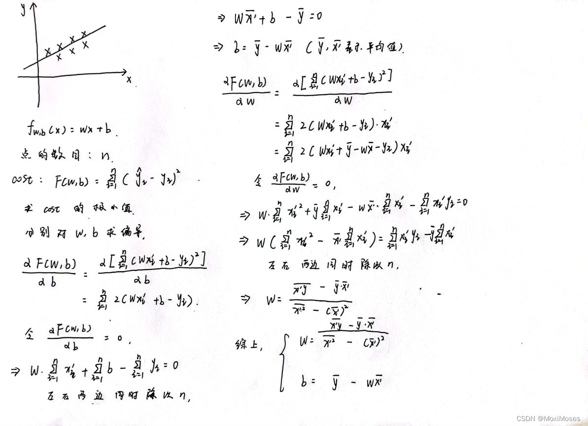
函数:f(x) = w * x + b
点的数目:n
代价函数:Σ〖(y_pred – y)〗^ 2
求代价函数的极小值:分别对w和b求偏导,并使偏导等于0
通过数学推导得到w和b,再通过w和b得到预测值。
2.线性回归的实现
先随机初始化10个0到10的整数,通过y = w * x + b得到正确的y值。
import numpy as np
import matplotlib.pyplot as plt


x = np.random.randint(0, 10, 10)
noise = np.random.normal(0, 3, 10)
y = x * 4 + 2 + noise
print(x)
print(y)
查看x和y的输出
[1 0 0 7 0 6 5 5 9 1]
[11.46684789  1.40615999  3.36165153 33.19321883  0.69712028 27.95070034
 23.70706215 16.91973905 32.46834576  9.23893302]
通过上面的数学推导得到的w和b,得到预测值y。
w = ((x * y).mean() - x.mean() * y.mean())/((x ** 2).mean() - x.mean() ** 2)
b = y.mean() - w * x.mean()

y_pred = w * x + b
print(y_pred)
查看预测值y的输出
[ 7.35226575  3.73196902  3.73196902 29.07404609  3.73196902 25.45374937
 21.83345264 21.83345264 36.31463954  7.35226575]
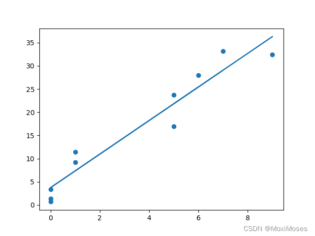
进行可视化,得到线性回归的函数。
3.线性回归的实现(矩阵思想)
先初始化以10为中心,1为标准差,数目为100个的正态分布,然后把x重塑成20 * 5,通过y = w * x + b得到20 * 1的y。
import numpy as np


x = np.random.normal(10, 1, 100)
x = np.reshape(x, (20, 5))
ww = [6, 4, 5, 3, 2]
noise = np.random.normal(0, 1, 20)
y = np.dot(x, ww) + 2 + noise
y = np.reshape(y, (20, 1))
print(x)
print(y)
查看x和y的输出
[[ 9.95146053 10.17499465  9.51867144 11.8196936  10.88985386]
 [10.40601393  8.38310707 10.76364137  9.24761749  9.80648308]
 [11.50482388  9.14348218 10.55028613  8.98980079 11.16103599]
 [10.6333975  11.09728315  9.41926497  9.60862883  9.20090143]
 [10.27741323 11.80732095  9.45074761  9.92468524 10.31514892]
 [ 9.82856057  9.84759775  8.39987339  8.211677    8.83044201]
 [10.99958994  9.46023601 10.53593686  9.93324605 10.45028666]
 [ 7.95285049 11.00248031  7.87872536 10.28643708 10.71743296]
 [ 9.35518031  9.93726987 10.05894546 10.87334025  9.87260173]
 [10.64853367 11.12896796  9.25825147  9.95188156 11.39075086]
 [12.19749206 10.09121693  8.88849207  9.05203882  9.20709902]
 [10.10989541 11.1550574   9.82845004  9.05581613 10.57649904]
 [10.29783321 10.82100454 10.86359896 12.05575292  9.51527671]
 [10.19964888 12.24978701  8.37146185  8.5140509   9.35818766]
 [11.59558143 10.10115058  9.69223148 10.58266507 10.01704913]
 [ 9.91734085  8.04875736 11.6616676  10.66029681 11.41891422]
 [11.29986005 11.07647544  9.74675509 10.15250374  8.65900066]
 [11.35587337  9.58548784 10.50846991 10.2332597  11.95795414]
 [ 8.83065153 11.04986874  8.75441082  9.59644547  9.26619456]
 [10.52308175 12.06750588 10.39531862  9.76549257 10.99956927]]
[[207.71548429]
 [199.78817148]
 [208.79960435]
 [205.08425979]
 [207.8221665 ]
 [185.03888373]
 [208.83907708]
 [185.83872255]
 [200.66164597]
 [209.13479127]
 [206.05043419]
 [205.34526174]
 [216.23265022]
 [198.67587884]
 [211.97840653]
 [206.31357248]
 [212.77174684]
 [216.2114928 ]
 [189.44338797]
 [216.73866285]]
通过以下公式:
w = w - learning_rate * (1/n) * (x * w + b - y) * x
b = b - learning_rate * (1/n) * (x * w + b - y)
得到w和b的值
# 学习速率
learning_rate = 1e-3


# 训练
def train(x, y):
    w = np.zeros((1, x.shape[1]))
    b = 0

    for epoch in range(10000):
        y_pred = np.dot(x, w.T) + b
        lost = y_pred - y
        # print(lost)

        w -= learning_rate * (1 / len(x)) * np.dot(lost.T, x)
        b -= learning_rate * (1 / len(x)) * lost.sum()
        loss = mse_loss(y, y_pred)
        if epoch % 1000 == 0:
            print("Epoch %d loss: %.3f" % (epoch, loss))

    return w, b


print("train")
w, b = train(x, y)
print(w)
print(b)
查看w和b的输出
[[6.23711088 4.07055996 4.88043289 3.12492006 1.84275656]]
0.4579777578042886
进行测试,得到预测值y。
# 测试
print("test")
y_pred = np.dot(x, w.T) + b
print(y_pred)
查看预测值输出
[[207.40245077]
 [198.98563628]
 [209.58337696]
 [204.90312247]
 [208.76764735]
 [184.77324442]
 [209.28996469]
 [185.19254779]
 [200.52065644]
 [209.4486846 ]
 [206.24502066]
 [204.67755179]
 [216.96092149]
 [198.64475922]
 [212.72949463]
 [206.34532229]
 [211.27449224]
 [215.60372129]
 [190.30366401]
 [216.73267863]]
4.搭建最简单的神经网络
import numpy as np


class Nerual_Network():
    def __init__(self):
        # weight
        self.w = np.random.normal(0, 1, 5)
        self.w = np.reshape(self.w, (1, 5))

        # bias
        self.b = 0

    def feedforward(self, x):
        y = np.dot(x, self.w.T) + self.b
        return y

    def train(self, x, y):
        # 学习速率
        learning_rate = 1e-3

        # 训练次数
        epoch = 10000

        for i in range(epoch):
            y_pred = np.dot(x, self.w.T) + self.b
            lost = y_pred - y

            self.w -= learning_rate * (1 / len(x)) * np.dot(lost.T, x)
            self.b -= learning_rate * (1 / len(x)) * lost.sum()

            if i % 1000 == 0:
                loss = mse_loss(y, y_pred)
                print("Epoch %d loss: %f" % (i, loss))

    def test(self, x):
        y = self.feedforward(x)
        return y


x = np.random.normal(10, 1, 100)
x = np.reshape(x, (20, 5))
ww = [6, 4, 5, 3, 2]
noise = np.random.normal(0, 1, 20)
y = np.dot(x, ww) + 2 + noise
y = np.reshape(y, (20, 1))
# print(x)
print(y)
print("train")
network = Nerual_Network()
network.train(x, y)
y_pred = network.test(x)
print(y_pred)
查看y和预测值的输出
[[205.30080299]
 [200.1836951 ]
 [186.04491518]
 [205.77013292]
 [211.82983047]
 [198.49851461]
 [208.42566702]
 [208.29517664]
 [197.67087052]
 [194.70403343]
 [199.95063503]
 [207.19674327]
 [208.28728383]
 [206.73747766]
 [201.26959204]
 [202.26798826]
 [213.51334817]
 [209.87308534]
 [197.43528161]
 [192.54548866]]
train
Epoch 0 loss: 43790.282428
Epoch 1000 loss: 2.366505
Epoch 2000 loss: 1.358675
Epoch 3000 loss: 1.120908
Epoch 4000 loss: 1.053084
Epoch 5000 loss: 1.027170
Epoch 6000 loss: 1.013942
Epoch 7000 loss: 1.005880
Epoch 8000 loss: 1.000571
Epoch 9000 loss: 0.996971
[[204.56872963]
 [200.28516158]
 [188.40788893]
 [207.04157146]
 [212.33578435]
 [198.79708815]
 [208.20117297]
 [207.49568625]
 [198.33166046]
 [194.35313567]
 [200.26159023]
 [206.52221361]
 [208.57481802]
 [204.54435871]
 [202.58427297]
 [201.95348356]
 [213.8315069 ]
 [209.42535055]
 [197.54027897]
 [190.82357382]]
总结
本周学习了CNN相关论文《ImageNet Classification with Deep ConvolutionalNeural Networks》,了解到AlexNet有很多开创的进展,使用了Relu替换了传统的sigmoid或tanh作为激活函数,大大加快了收敛,减少了模型训练耗时;使用了Dropout,提高了模型的准确度,减少过拟合;使用了2种数据扩增技术,大幅增加了训练数据,增加模型鲁棒性,减少过拟合。下周我会继续阅读CNN的相关论文,并对项目的框架进行展开学习,用代码实现CNN手写数字识别。


 614
614


 被折叠的 条评论
为什么被折叠?
被折叠的 条评论
为什么被折叠?
 到【灌水乐园】发言


