some record in matlab code

(shift+f3)可以切换英文大小写！！！
1—add path in the matlab:

addpath('utilities');
addpath('solver');

2—- matlab function handle
这是一种间接调用函数的形式，但是很高效，
handle = @functionname
handle = @(arglist)anonymous_function

sqr = @(x) x.^2;
sqr(20)

3—about the sparse web and CS
http://www.cnblogs.com/daniel-D/p/3222576.html
这里面引用的coursera 上面的内容

http://www.cvchina.info/2010/06/01/sparse-representation-vector-matrix-tensor-1/

http://www.cvchina.info/tag/%E5%8E%8B%E7%BC%A9%E6%84%9F%E7%9F%A5/

4—Hadamard product (matrices)
For two matrices of the same dimensions, there is the Hadamard product, also known as the element-wise product, pointwise product, entrywise product and the Schur product.[24] For two matrices A and B of the same dimensions, the Hadamard product A ○ B is a matrix of the same dimensions, the i, j element of A is multiplied with the i, j element of B, that is:

\left(\mathbf{A} \circ \mathbf{B}\right){ij} = A{ij}B_{ij},,

The Frobenius inner product, sometimes denoted A : B, is the component-wise inner product of two matrices as though they are vectors. It is also the sum of the entries of the Hadamard product. Explicitly,

\mathbf{A}:\mathbf{B}=\sum_{i,j} A_{ij} B_{ij} = \mathrm{vec}(\mathbf{A})^\mathsf{T} \mathrm{vec}(\mathbf{B}) = \mathrm{tr}(\mathbf{A}^\mathsf{T} \mathbf{B}) = \mathrm{tr}(\mathbf{A} \mathbf{B}^\mathsf{T}),
where “tr” denotes the trace of a matrix and vec denotes vectorization. This inner product induces the Frobenius norm.

5—image reconstruction toolbox
http://web.eecs.umich.edu/~fessler/code/

6——Nonuniform Fast Fourier Transforms (NUFFT)
some website:
http://research.engineering.uiowa.edu/cbig/content/accurate-nufft-using-optimized-interpolator-and-scale-factors
下图在1D数据中，显示了FFT与NUFFT的区别：

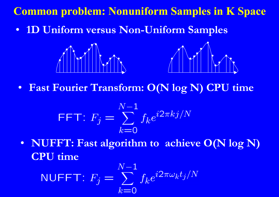
一个均匀采样，一个非均匀采样
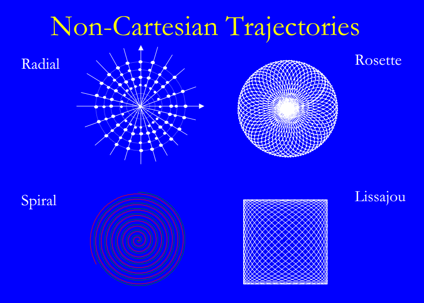
下图显示在医学图像处理中的采样方式：

下图在图像处理中的对比残差：

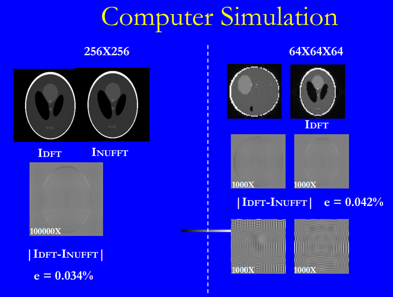
上图中的残差计算，没有明白为啥右下角的图像时那种条纹。。。。

重在应用MRI

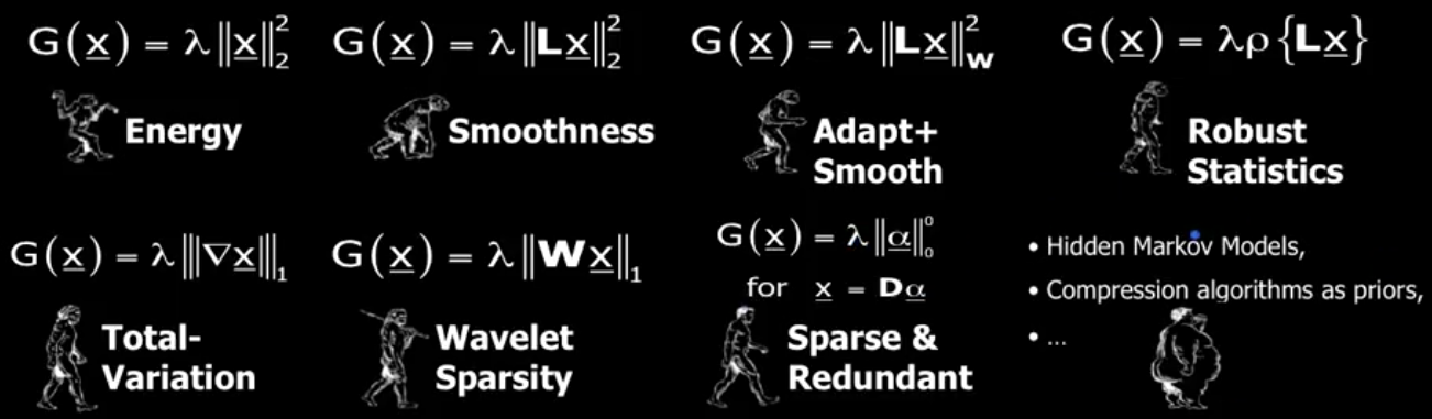
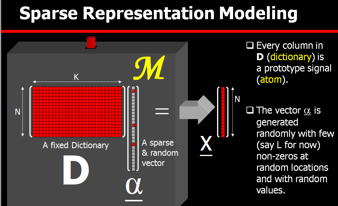
7—-sparse coding 和 sparse representation 的区别
稀疏编码是获得稀疏表示的一种途径-zhihua zhou
S R 广泛应用于 图像恢复、去模糊、inpainting、物体检测等等，最近几年非常热，大量文章出现。
最早的一篇文章是1996年的Nature 上的一篇文章
emergence of simple
在线性表达上进行了稀疏约束，得到了一下表征图像固有特征的基函数（不一定正交） localized\ oriented \ bandpass

Elad的一个slide 有详细讲解SP的问题及理论，非常好
Ecole_Polytechnique_MMSE_April_2009.ppt
稀疏表示的模型如图

另外，最近稀疏表示的论文，可以参考最近出来的一个survey，A Survey of Sparse Representation: Algorithms and Applications， 内容比较详尽，总结了SP发展中的sparse 约束的5种不同范数类型：

1. L0-范数
2. Lp-范数
3. L1-范数
4. L2,1-范数
5. L2-范数

---

将求解的上述不同约束的SP算法归结了4类，

1. greedy strategy approximation，常见的为Matching pursuit, Orthogonal Matching Pursuit

2. constrained optimization

3. proximity algorithm-based optimization
4. homotopu algorithm-based sparse representation

http://arxiv.org/pdf/1506.07515v1.pdf

8—–steepest descent method 最速梯度下降法
在看FISTA的方法的时候，发现algorithm 的步骤跟程序稍微有一点不匹配，按照流程修改之后就发现是错的，原来隐藏在里面一个梯度和导数的关系

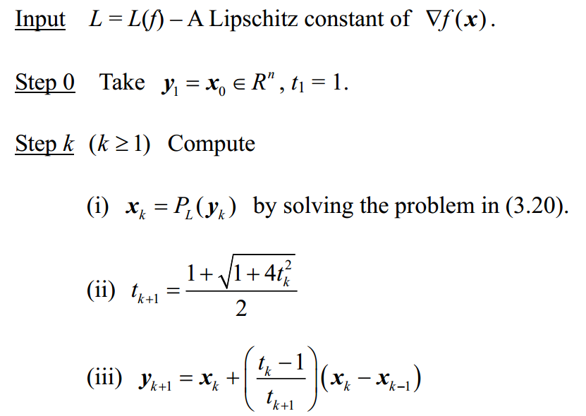
在程序中的5-6行，改的是错误的

ck = yk - 2*Li*A'*(A*yk-yn);
thk1 = (max(abs(ck)-alp,0)).*sign(ck);
tk1 = 0.5 + 0.5*sqrt(1+4*tk^2);
tt = (tk-1)/tk1;
yk = thk1 +tt*(thk1-thk);
%yk = thk1 -tt*(thk1-thk);% this is right
tk = tk1;
thk = thk1;

原来是用了最速下降法（steepest descent method），最速下降的方向是负梯度方向：-g(k)/|g(k)|
归结为： x(k+1)=x(k)-a*g(k)，g(k)是x(k)的梯度
具体参考博客
自己在优化方面需要好好看，程序都看不懂！！

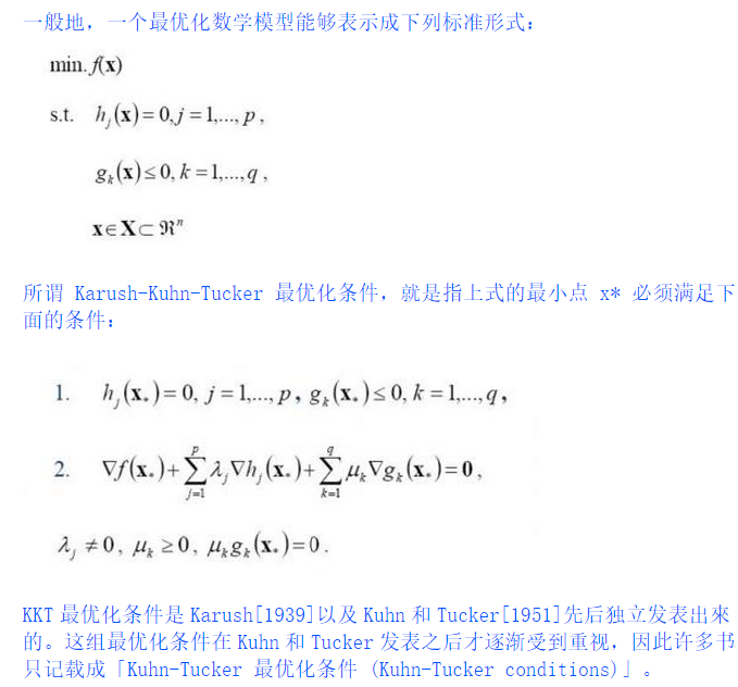
关于范数性质中，成立的两个等式

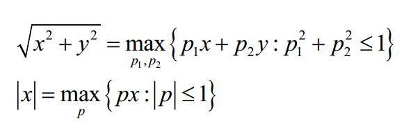
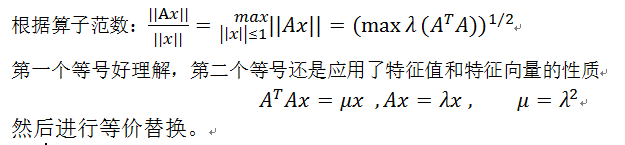
第二个等式是LP问题，可以求解

常用： KKT condition