Python处理时空数据常用库案例及练习

qazwsxpy

已于 2022-12-01 18:44:50 修改

阅读量1.7k

点赞数

分类专栏：地球科学文章标签： python arcgis 开发语言

于 2022-12-01 18:36:56 首次发布

本文链接：https://blog.csdn.net/qazwsxpy/article/details/128135721

版权

地球科学专栏收录该内容

5 篇文章 10 订阅

订阅专栏

本文完整代码、数据集下载、在线运行可以访问这个链接：时空数据Python常用包案例
配套习题与答案可以访问这个链接：时空数据Python常用包案例 - 实操练习题（附答案）

Python处理时空数据会用到如下常用库：

库	作用
GeoPands	geopandas是建立在GEOS、GDAL、PROJ等开源地理空间计算相关框架之上的，类似pandas语法风格的空间数据分析Python库，其目标是尽可能地简化Python中的地理空间数据处理，减少对Arcgis、PostGIS等工具的依赖，使得处理地理空间数据变得更加高效简洁，打造纯Python式的空间数据处理工作流。
Shapely	shapely是一个BSD授权的Python包。是专门做图形计算,用于操作和分析笛卡尔坐标系中的几何对象 ,基本上图形线段，点的判断包里都有，shapely里主要由Point，LineString，Polygon这三类组成。
pyproj	pyproj可以方便地进行坐标转换，包含了地理坐标系、坐标系、ECEF、BLH、ECI，ENU等坐标系，简单易用
Fiona	Fiona可以读和写地理数据文件，从而帮助Python程序员将地理信息系统与其他计算机系统结合起来。Fiona包含连接地理空间数据抽象库（GDAL）的扩展模块。它专注于以标准的Python IO风格读写数据，并依赖于熟悉的Python类型和协议，如文件、字典、映射和迭代器，而不是GDAL的OpenGIS参考实现（OGR）的特定类。
rasterio	Rasterio使用更少的非惯用扩展类和更多的惯用python类型和协议表达gdal的数据模型，同时执行与gdal的python绑定一样快

以下分别罗列这些库的简单示例：

GeoPands

%matplotlib inline
import numpy as np
import matplotlib.pyplot as plt
from geopandas import GeoSeries, GeoDataFrame, read_file
from shapely.geometry import Point
from pandas import Series

下载纽约市各区的边界数据：Bytes of the Big Apple

boros = read_file('/home/mw/input/st201516189/nybb.shp')

boros.set_index('BoroCode', inplace=True)
boros.sort_index(inplace=True)
boros

	BoroName	Shape_Leng	Shape_Area	geometry
BoroCode
1	Manhattan	358408.460709	6.364467e+08	MULTIPOLYGON (((981219.056 188655.316, 980940....
2	Bronx	464400.198868	1.186973e+09	MULTIPOLYGON (((1012821.806 229228.265, 101278...
3	Brooklyn	741185.900596	1.937597e+09	MULTIPOLYGON (((1021176.479 151374.797, 102100...
4	Queens	897040.298576	3.045168e+09	MULTIPOLYGON (((1029606.077 156073.814, 102957...
5	Staten Island	330466.075042	1.623827e+09	MULTIPOLYGON (((970217.022 145643.332, 970227....

boros.reset_index(inplace=True)
boros.set_index('BoroName', inplace=True)
boros

	BoroCode	Shape_Leng	Shape_Area	geometry
BoroName
Manhattan	1	358408.460709	6.364467e+08	MULTIPOLYGON (((981219.056 188655.316, 980940....
Bronx	2	464400.198868	1.186973e+09	MULTIPOLYGON (((1012821.806 229228.265, 101278...
Brooklyn	3	741185.900596	1.937597e+09	MULTIPOLYGON (((1021176.479 151374.797, 102100...
Queens	4	897040.298576	3.045168e+09	MULTIPOLYGON (((1029606.077 156073.814, 102957...
Staten Island	5	330466.075042	1.623827e+09	MULTIPOLYGON (((970217.022 145643.332, 970227....

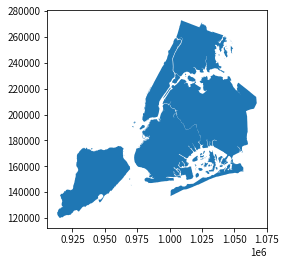
plt.figure(figsize=(8, 8))
boros.plot()

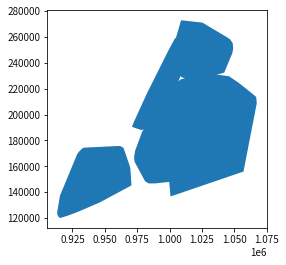
plt.figure(figsize=(8, 8))
boros.plot(alpha=0.0)
boros.geometry.convex_hull.plot()

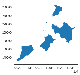
plt.figure(figsize=(8, 8))
eroded = boros.geometry.buffer(-5280)
boros.plot(alpha=0.0)
eroded.plot()

eroded.area

BoroName
Manhattan        1.128785e+07
Bronx            3.371876e+08
Brooklyn         6.711072e+08
Queens           1.301421e+09
Staten Island    7.263977e+08
dtype: float64

boros.geometry.area

BoroName
Manhattan        6.364464e+08
Bronx            1.186974e+09
Brooklyn         1.937596e+09
Queens           3.045168e+09
Staten Island    1.623829e+09
dtype: float64

inland = 100.0 * eroded.area / boros.geometry.area

boros['inland_fraction'] = inland

boros

	BoroCode	Shape_Leng	Shape_Area	geometry	inland_fraction
BoroName
Manhattan	1	358408.460709	6.364467e+08	MULTIPOLYGON (((981219.056 188655.316, 980940....	1.773574
Bronx	2	464400.198868	1.186973e+09	MULTIPOLYGON (((1012821.806 229228.265, 101278...	28.407326
Brooklyn	3	741185.900596	1.937597e+09	MULTIPOLYGON (((1021176.479 151374.797, 102100...	34.636066
Queens	4	897040.298576	3.045168e+09	MULTIPOLYGON (((1029606.077 156073.814, 102957...	42.737251
Staten Island	5	330466.075042	1.623827e+09	MULTIPOLYGON (((970217.022 145643.332, 970227....	44.733620

让我们创建一个正常的pandasSeries，其中包含2010年人口普查中每个区的人口值。

population = Series({'Manhattan': 1585873, 'Bronx': 1385108, 'Brooklyn': 2504700,
                     'Queens': 2230722, 'Staten Island': 468730})
population

Manhattan        1585873
Bronx            1385108
Brooklyn         2504700
Queens           2230722
Staten Island     468730
dtype: int64

boros['population'] = population
boros

	BoroCode	Shape_Leng	Shape_Area	geometry	inland_fraction	population
BoroName
Manhattan	1	358408.460709	6.364467e+08	MULTIPOLYGON (((981219.056 188655.316, 980940....	1.773574	1585873
Bronx	2	464400.198868	1.186973e+09	MULTIPOLYGON (((1012821.806 229228.265, 101278...	28.407326	1385108
Brooklyn	3	741185.900596	1.937597e+09	MULTIPOLYGON (((1021176.479 151374.797, 102100...	34.636066	2504700
Queens	4	897040.298576	3.045168e+09	MULTIPOLYGON (((1029606.077 156073.814, 102957...	42.737251	2230722
Staten Island	5	330466.075042	1.623827e+09	MULTIPOLYGON (((970217.022 145643.332, 970227....	44.733620	468730

boros['pop_density'] = boros['population'] / boros.geometry.area * 5280 ** 2

boros.sort_values('pop_density', ascending=False)

The history saving thread hit an unexpected error (OperationalError('attempt to write a readonly database')).History will not be written to the database.

	BoroCode	Shape_Leng	Shape_Area	geometry	inland_fraction	population	pop_density
BoroName
Manhattan	1	358408.460709	6.364467e+08	MULTIPOLYGON (((981219.056 188655.316, 980940....	1.773574	1585873	69466.335981
Brooklyn	3	741185.900596	1.937597e+09	MULTIPOLYGON (((1021176.479 151374.797, 102100...	34.636066	2504700	36037.963313
Bronx	2	464400.198868	1.186973e+09	MULTIPOLYGON (((1012821.806 229228.265, 101278...	28.407326	1385108	32531.958243
Queens	4	897040.298576	3.045168e+09	MULTIPOLYGON (((1029606.077 156073.814, 102957...	42.737251	2230722	20422.174910
Staten Island	5	330466.075042	1.623827e+09	MULTIPOLYGON (((970217.022 145643.332, 970227....	44.733620	468730	8047.300267

boros['simplified'] = boros.geometry.simplify(1000)
boros

	BoroCode	Shape_Leng	Shape_Area	geometry	inland_fraction	population	pop_density	simplified
BoroName
Manhattan	1	358408.460709	6.364467e+08	MULTIPOLYGON (((981219.056 188655.316, 980940....	1.773574	1585873	69466.335981	MULTIPOLYGON (((981219.056 188655.316, 980873....
Bronx	2	464400.198868	1.186973e+09	MULTIPOLYGON (((1012821.806 229228.265, 101278...	28.407326	1385108	32531.958243	MULTIPOLYGON (((1012821.806 229228.265, 101250...
Brooklyn	3	741185.900596	1.937597e+09	MULTIPOLYGON (((1021176.479 151374.797, 102100...	34.636066	2504700	36037.963313	MULTIPOLYGON (((1021176.479 151374.797, 102003...
Queens	4	897040.298576	3.045168e+09	MULTIPOLYGON (((1029606.077 156073.814, 102957...	42.737251	2230722	20422.174910	MULTIPOLYGON (((1029606.077 156073.814, 103074...
Staten Island	5	330466.075042	1.623827e+09	MULTIPOLYGON (((970217.022 145643.332, 970227....	44.733620	468730	8047.300267	MULTIPOLYGON (((970217.022 145643.332, 970547....

boros.set_geometry('simplified', inplace=True)
boros

	BoroCode	Shape_Leng	Shape_Area	geometry	inland_fraction	population	pop_density	simplified
BoroName
Manhattan	1	358408.460709	6.364467e+08	MULTIPOLYGON (((981219.056 188655.316, 980940....	1.773574	1585873	69466.335981	MULTIPOLYGON (((981219.056 188655.316, 980873....
Bronx	2	464400.198868	1.186973e+09	MULTIPOLYGON (((1012821.806 229228.265, 101278...	28.407326	1385108	32531.958243	MULTIPOLYGON (((1012821.806 229228.265, 101250...
Brooklyn	3	741185.900596	1.937597e+09	MULTIPOLYGON (((1021176.479 151374.797, 102100...	34.636066	2504700	36037.963313	MULTIPOLYGON (((1021176.479 151374.797, 102003...
Queens	4	897040.298576	3.045168e+09	MULTIPOLYGON (((1029606.077 156073.814, 102957...	42.737251	2230722	20422.174910	MULTIPOLYGON (((1029606.077 156073.814, 103074...
Staten Island	5	330466.075042	1.623827e+09	MULTIPOLYGON (((970217.022 145643.332, 970227....	44.733620	468730	8047.300267	MULTIPOLYGON (((970217.022 145643.332, 970547....

boros._geometry_column_name

'simplified'

plt.figure(figsize=(8, 8))
boros.plot()

Shapely

演示例子基于 Shapely user manual。

import matplotlib.pyplot as plt
from shapely.geometry import LineString
from descartes.patch import PolygonPatch
%matplotlib inline
BLUE = 'lightblue'
GRAY = 'lightgray'

def plot_line(ax, ob):
    x, y = ob.xy
    ax.plot(x, y, color=GRAY, linewidth=3, solid_capstyle='round', zorder=1)

扩大一条线

在直线周围的正缓冲区生成多边形。

ax = plt.subplot(111)
line = LineString([(0, 0), (1, 1), (0, 2), (2, 2), (3, 1), (1, 0)])
plot_line(ax, line)
dilated = line.buffer(0.5, cap_style=3)
patch1 = PolygonPatch(dilated, fc=BLUE, ec=BLUE, alpha=0.5, zorder=2)
ax.add_patch(patch1)
ax.set_xlim(-1, 4)
ax.set_ylim(-1, 3)
plt.show()

/opt/conda/lib/python3.9/site-packages/descartes/patch.py:63: ShapelyDeprecationWarning: The array interface is deprecated and will no longer work in Shapely 2.0. Convert the '.coords' to a numpy array instead.
  concatenate([asarray(t.exterior)[:, :2]] +
/opt/conda/lib/python3.9/site-packages/descartes/patch.py:64: ShapelyDeprecationWarning: The array interface is deprecated and will no longer work in Shapely 2.0. Convert the '.coords' to a numpy array instead.
  [asarray(r)[:, :2] for r in t.interiors])

削弱多边形

在多边形内部的特定距离的区域生成负的缓冲区

ax = plt.subplot(111)
patch2a = PolygonPatch(dilated, fc=GRAY, ec=GRAY, alpha=0.5, zorder=1)
ax.add_patch(patch2a)
eroded = dilated.buffer(-0.3)
patch2b = PolygonPatch(eroded, fc=BLUE, ec=BLUE, alpha=0.5, zorder=2)
ax.add_patch(patch2b)
ax.set_xlim(-1, 4)
ax.set_ylim(-1, 3)

plt.show()

所有的Shapely对象都有一个__geo_interface__属性，用来返回对象的GeoJSON表示

eroded.__geo_interface__

{'type': 'Polygon',
 'coordinates': (((0.5050252531694168, 0.7878679656440357),
   (0.5247963548222736, 0.8096820147509064),
   (0.5423341025042161, 0.8333289300941193),
   (0.557469598117959, 0.8585809789522008),
   (0.5700570785668386, 0.8851949702904731),
   (0.5799753195331152, 0.9129145968236613),
   (0.5871288029344217, 0.9414729033951615),
   (0.5914486368151116, 0.9705948579011319),
   (0.5928932188134526, 1.0),
   (0.5914486368151116, 1.0294051420988681),
   (0.5871288029344217, 1.0585270966048386),
   (0.5799753195331152, 1.0870854031763386),
   (0.5700570785668386, 1.1148050297095269),
   (0.5574695981179589, 1.1414190210477992),
   (0.5423341025042161, 1.1666710699058807),
   (0.5247963548222736, 1.1903179852490937),
   (0.5050252531694168, 1.2121320343559643),
   (-0.13621380708870784, 1.8533710946140889),
   (-0.15432241630904883, 1.8733508659857347),
   (-0.165993097635207, 1.8890869581181033),
   (-0.17606517469008098, 1.9058912034750313),
   (-0.18444164786567485, 1.923601767987596),
   (-0.19104184714626118, 1.9420480892379615),
   (-0.1958022090047325, 1.961052519068703),
   (-0.1986768885541129, 1.9804320344316715),
   (-0.19963820105888225, 2.0000000000000013),
   (-0.19867688855411278, 2.0195679655683296),
   (-0.19580220900473197, 2.0389474809312995),
   (-0.1910418471462608, 2.0579519107620396),
   (-0.184441647865674, 2.0763982320124064),
   (-0.1760651746900811, 2.0941087965249685),
   (-0.16599309763520584, 2.110913041881898),
   (-0.15432241630904767, 2.1266491340142664),
   (-0.14116552575261862, 2.141165525752619),
   (-0.12664913401426514, 2.154322416309049),
   (-0.11091304188189907, 2.165993097635205),
   (-0.09410879652496867, 2.176065174690081),
   (-0.07639823201240363, 2.184441647865675),
   (-0.05795191076204117, 2.1910418471462605),
   (-0.03894748093129574, 2.1958022090047327),
   (-0.019567965568329727, 2.198676888554113),
   (0.00736458663268156, 2.2),
   (1.9926354133673185, 2.2),
   (2.0195679655683296, 2.198676888554113),
   (2.0389474809312977, 2.195802209004732),
   (2.0579519107620405, 2.1910418471462605),
   (2.076398232012405, 2.1844416478656745),
   (2.094108796524969, 2.176065174690081),
   (2.1109130418818958, 2.1659930976352073),
   (2.1266491340142686, 2.1543224163090464),
   (2.146628905385912, 2.1362138070887076),
   (3.1361377664312835, 1.1467049460433356),
   (3.1544954989456087, 1.1264211218730886),
   (3.1663014116038086, 1.1104309727779462),
   (3.1764586953242713, 1.0933460663046861),
   (3.1848666558813163, 1.0753357736627291),
   (3.191441940963334, 1.0565786398766723),
   (3.196119366485863, 1.0372606137803255),
   (3.198852562793971, 1.0175732046130626),
   (3.199614434347804, 0.9977115834930848),
   (3.198397428334199, 0.9778726485886986),
   (3.1952136095414945, 0.9582530731683895),
   (3.190094540755259, 0.9390473558805693),
   (3.1830909698606353, 0.9204458925913018),
   (3.1742723267532176, 0.9026330888950328),
   (3.163726035045817, 0.8857855320098248),
   (3.1515566453945416, 0.8700702401801029),
   (3.1378847990359287, 0.855643006941387),
   (3.122846031810121, 0.8426468566611727),
   (3.106589430526412, 0.8312106266669667),
   (3.082759447896349, 0.8177729261981954),
   (1.0894427190999916, -0.1788854381999832),
   (0.9105572809000084, -0.26832815729997483),
   (0.7980190881121922, -0.04325177172434258),
   (0.7833473608114292, -0.01723340589287306),
   (0.7661610106538479, 0.00719699137751828),
   (0.7466304145107607, 0.029797229359091987),
   (0.7249491889345605, 0.05034326060704983),
   (0.7013322707411517, 0.0686314020537353),
   (0.6760137862339635, 0.08448035422059508),
   (0.6492447301929902, 0.0977329985304437),
   (0.6212904776381997, 0.10825795490237844),
   (0.5924281530344432, 0.11595088418812699),
   (0.562943883018249, 0.1207355225381277),
   (0.5331299598815951, 0.1225644374431531),
   (0.5032819439324578, 0.12141949795646018),
   (0.4736957334578889, 0.11731205443491916),
   (0.44466463133653505, 0.1102828260172578),
   (0.4164764373807375, 0.10040149695490608),
   (0.3894105952332769, 0.08776602579721349),
   (0.36373542210299836, 0.0725016742794331),
   (0.3397054488023335, 0.05475976554058912),
   (0.3175588964562533, 0.034716183981634285),
   (0.0, -0.28284271247461895),
   (-0.2828427124746189, -1.2194129823122584e-17),
   (0.5050252531694168, 0.7878679656440357)),
  ((1.1791768829675937, 0.9124703578563456),
   (1.167822181791025, 0.8850237484926038),
   (1.1592372562731246, 0.8565888287946866),
   (1.153506262111692, 0.8274443385727507),
   (1.1506853786890343, 0.7978759733644631),
   (1.150802258360708, 0.768173583839086),
   (1.1538557553869733, 0.738628334469932),
   (1.1598159371641703, 0.7095298493279585),
   (1.1686243776459189, 0.6811633729755036),
   (1.1801947300778144, 0.6538069742911624),
   (1.1944135734312558, 0.6277288206359439),
   (1.2111415242390444, 0.6031845490813206),
   (1.2302146029337317, 0.5804147604683105),
   (1.2514458412948701, 0.5596426608626514),
   (1.2746271152477977, 0.5410718735262403),
   (1.2995311850475284, 0.5248844428534918),
   (1.3259139228483745, 0.5112390498394856),
   (1.3535167058230457, 0.5002694565731836),
   (1.3820689513721203, 0.49208319500392983),
   (1.411290769571924, 0.4867605128348993),
   (1.4408957068595831, 0.4843535868766154),
   (1.4705935540596553, 0.4848860115718198),
   (1.5000931912260107, 0.4883525677055459),
   (1.529105441411753, 0.49471927356766804),
   (1.5573459053924448, 0.5039237180663951),
   (1.5845377495546138, 0.5158756725272857),
   (2.290081561608991, 0.8686475785544743),
   (2.316099927440461, 0.8833193058552374),
   (2.3405303247108518, 0.9005056560128187),
   (2.3631305626924255, 0.9200362521559059),
   (2.3836765939403834, 0.9417174777321062),
   (2.401964735387069, 0.965334395925515),
   (2.4178136875539287, 0.9906528804327032),
   (2.4310663318637773, 1.0174219364736765),
   (2.441591288235712, 1.045376189028467),
   (2.4492842175214604, 1.0742385136322234),
   (2.454068855871461, 1.1037227836484176),
   (2.4558977707764864, 1.1335367067850717),
   (2.4547528312897935, 1.163384722734209),
   (2.450645387768253, 1.1929709332087777),
   (2.4436161593505914, 1.2220020353301315),
   (2.4337348302882393, 1.250190229285929),
   (2.421099359130547, 1.2772560714333898),
   (2.4058350076127666, 1.3029312445636683),
   (2.3880930988739224, 1.326961217864333),
   (2.368049517314968, 1.3491077702104133),
   (2.005025253169417, 1.7121320343559643),
   (1.9832112040625463, 1.731903136008821),
   (1.9595642887193332, 1.7494408836907636),
   (1.9343122398612518, 1.7645763793045064),
   (1.9076982485229794, 1.777163859753386),
   (1.8799786219897912, 1.7870821007196627),
   (1.851420315418291, 1.7942355841209692),
   (1.8222983609123207, 1.798555418001659),
   (1.7928932188134525, 1.8),
   (1.2071067811865475, 1.8),
   (1.1777016390876776, 1.798555418001659),
   (1.1485796845817073, 1.7942355841209687),
   (1.1200213780102073, 1.7870821007196622),
   (1.0923017514770192, 1.7771638597533854),
   (1.0656877601387469, 1.764576379304506),
   (1.0404357112806655, 1.7494408836907627),
   (1.0167887959374526, 1.7319031360088202),
   (0.9949747468305823, 1.7121320343559634),
   (0.9752036451777255, 1.6903179852490926),
   (0.9576658974957832, 1.6666710699058798),
   (0.9425304018820404, 1.6414190210477984),
   (0.9299429214331612, 1.614805029709526),
   (0.9200246804668846, 1.587085403176338),
   (0.9128711970655782, 1.5585270966048377),
   (0.9085513631848883, 1.5294051420988675),
   (0.9071067811865474, 1.4999999999999993),
   (0.9085513631848885, 1.4705948579011314),
   (0.9128711970655785, 1.441472903395161),
   (0.9200246804668849, 1.412914596823661),
   (0.9299429214331616, 1.385194970290473),
   (0.9425304018820411, 1.3585809789522005),
   (0.9576658974957839, 1.3333289300941193),
   (0.9752036451777265, 1.3096820147509063),
   (0.9949747468305832, 1.2878679656440357),
   (1.1362138070887098, 1.1466289053859091),
   (1.1543224163090473, 1.126649134014267),
   (1.1659930976352069, 1.1109130418818967),
   (1.1760651746900799, 1.0941087965249705),
   (1.1844416478656743, 1.076398232012405),
   (1.1910418471462612, 1.0579519107620383),
   (1.1958022090047324, 1.0389474809312975),
   (1.1986768885541128, 1.01956796556833),
   (1.1996382010588822, 1.0),
   (1.1986768885541128, 0.9804320344316703),
   (1.1958022090047324, 0.9610525190687029),
   (1.191041847146261, 0.9420480892379607),
   (1.184441647865674, 0.9236017679875939),
   (1.1791768829675937, 0.9124703578563456)))}

pyproj

pyproj是古老的PROJ.4库的一个python接口。地理坐标的转换可以由一个`Proj’实例完成，它可以用几种不同的方式定义。

从经度、纬度到地图坐标的转换是对一个Proj实例的调用，我们已经通过它的EPSG代码将其初始化。

import warnings
warnings.filterwarnings('ignore')

from __future__ import print_function
from pyproj import Proj, transform
epsg32618 = Proj(init='epsg:32618')
lat, lon = 40.78, -73.97
x, y = epsg32618(lon, lat)
x, y

(586912.663584656, 4514845.724134378)

反向转换是由同一对象用关键字参数inverse=True完成的:

epsg32618(x, y, inverse=True)

(-73.97, 40.779999999999994)

我们可以通过区域来初始化一个UTM投影。18区等同于上面的EPSG，所以我们应该得到同样的结果:

utm18 = Proj(proj="utm", zone="18")
print(utm18(lon, lat))

(586912.663584656, 4514845.724134378)

可以使用"+proj=utm +zone=18 "这样的字符串（这与PROJ.4`命令行参数兼容）.

utm18 = Proj("+proj=utm +zone=18")
print(utm18(lon, lat))

(586912.663584656, 4514845.724134378)

我们可以进行基准点转换以及地图投影。需要创建一个以NAD27为基准的投影。

nad27 = Proj(proj="utm", zone="18", ellps="clrk66", datum="NAD27")
print(nad27(lon, lat))

(586914.9904254216, 4514634.228909359)

我们也可以直接在两个参考框架之间做这种转换:

old_x, old_y = transform(utm18, nad27, x, y)
old_x, old_y

(586878.5100284991, 4514633.864793612)

包括Fiona、rasterio和GeoPandas在内的库使用了一个轻量级的python参数字典，当需要进行转换时可以传递给Proj构造函数。
这里我们使用相当于EPSG:2263的明确参数（纽约州平面长岛，美国英尺）:

crs = {'lon_0': -74, 'datum': 'NAD83', 'y_0': 0, 'no_defs': True, 'proj': 'lcc',
       'x_0': 300000, 'units': 'us-ft', 'lat_2': 41.03333333333333,
       'lat_1': 40.66666666666666, 'lat_0': 40.16666666666666}
nyc = Proj(**crs)
print(nyc(lon, lat))

(992558.4426667999, 223453.30015578947)

Fiona

我们将使用由Mapzen从OpenStreetMap 中提取的德克萨斯州奥斯汀水域的形状文件.

from __future__ import print_function
import os
import numpy as np
import matplotlib.pyplot as plt
import fiona
%matplotlib inline

data_dir = os.path.join(os.path.abspath('..'), 'data')
input_file = os.path.join(data_dir, 'austin-osm', '/home/mw/input/st201516189/austin_texas_osm_waterareas.shp')
if os.path.exists(input_file):
    print('Input file:', input_file)
else:
    print('Please download the tutorial data or fix the path!')

Input file: /home/mw/input/st201516189/austin_texas_osm_waterareas.shp

首先使用Fiona的“open（）”函数以“r”模式打开读取GIS矢量文件。该函数会返回一个打开的“集合”对象。

c = fiona.open(input_file, 'r')
c

<open Collection '/home/mw/input/st201516189/austin_texas_osm_waterareas.shp:austin_texas_osm_waterareas', mode 'r' at 0x7f0747f3edc0>

len(c)

“集合”具有只读驱动程序属性，该属性命名用于打开矢量文件的OGR格式驱动程序。

c.driver

'ESRI Shapefile'

集合向量数据的坐标参考系（CRS）通过只读CRS属性访问，该属性由PROJ.4个参数映射表示

c.crs

{'init': 'epsg:4326'}

fiona.crs模块提供3个功能来帮助这些映射。

from fiona.crs import to_string, from_string, from_epsg

to_string（）将映射转换为PROJ.4类型的字符串：

print(to_string(c.crs))

+init=epsg:4326

from_string（）用于执行反向操作。

from_string("+datum=WGS84 +ellps=WGS84 +no_defs +proj=longlat")

{'datum': 'WGS84', 'ellps': 'WGS84', 'no_defs': True, 'proj': 'longlat'}

`from_epsg（）用于从epsg代码映射到CRS快捷方式。

from_epsg(3857)

{'init': 'epsg:3857', 'no_defs': True}

Fiona的Collection的作用很像一个打开的Python文件，但其是在记录进行迭代而非在行上迭代。

rec = c.next()

<ipython-input-12-eb6a7f87923f>:1: FionaDeprecationWarning: Collection.__next__() is buggy and will be removed in Fiona 2.0. Switch to `next(iter(collection))`.
  rec = c.next()

从集合中获得的记录是一个Python dict，其结构与GeoJSON Feature完全相同。Fiona的记录是自我描述的；其字段的名称包含在数据结构中，字段中的值根据记录类型正确键入。
例如，数字字段值是int和float类型的实例，而不是字符串。

rec.keys()

dict_keys(['type', 'id', 'properties', 'geometry'])

记录具有“properties”键。其对应的值是映射。属性映射的键与其集合架构中的属性映射键相同。

rec['properties']

OrderedDict([('id', 1),
             ('osm_id', -2439371.0),
             ('name', 'Soil Conservation Service Site 14 Reservoir'),
             ('type', 'water'),
             ('area', 3.02358e-05)])

记录具有几何键。它的对应值是一个带有类型和坐标键的映射。因为坐标只是元组、元组列表，或者元组的列表，所以类型告诉你如何解释它们。

rec['geometry'].keys()

dict_keys(['type', 'coordinates'])

rec['geometry']['type']

'Polygon'

for poly in rec['geometry']['coordinates']:
    coords = np.array(poly).squeeze()
    print(coords.shape)
    plt.plot(coords[:,0], coords[:,1])
plt.gca().set_aspect('equal')

(110, 2)
(11, 2)

接下来，我们将提取定义Lake Travis海岸线的外部多边形。

lake_travis = [rec for rec in c if rec['properties']['name'] == 'Lake Travis']
outer = lake_travis[0]['geometry']['coordinates']
coords = np.array(outer[0][0]).squeeze()
plt.plot(coords[:,0], coords[:,1], fillstyle='full')
plt.gca().set_aspect('equal')

我们没有在上下文管理器（“with”语句）中打开该文件，这是一个很好的做法，因此我们需要显式关闭该文件。

c.close()

筛选(filtering)

对于某些矢量数据格式，空间索引伴随着数据文件，允许有效的边界框搜索。集合的filter()方法返回与给定(minx，miny，maxx，maxy)边界框相交的记录的迭代器。集合自身的坐标参考系统（在本例中为WGS84经度/纬度）用于解释框的值。

（这次我们将使用上下文管理器，以便文件自动关闭。）

with fiona.open(input_file, 'r') as c:
    hits = c.filter(bbox=(-98.210438, 30.357799, -97.884216, 30.568691))
    print(len(list(hits)))

rasterio

National Weather Service radar mosaic显示了美国48个大陆州的情况。但不巧的是，它是以未投影的纬度/纬度坐标显示的。

在这个例子中，我们将使用rasterio将图像重新投影到一个更标准的等面积投影中。

基于一篇使用GDALwarp的博文和rasterio reproject范例。

!pip install -U pyOpenSSL -i https://mirrors.cloud.tencent.com/pypi/simple

Looking in indexes: https://mirrors.cloud.tencent.com/pypi/simple
Requirement already satisfied: pyOpenSSL in /opt/conda/lib/python3.9/site-packages (22.1.0)
Requirement already satisfied: cryptography<39,>=38.0.0 in /opt/conda/lib/python3.9/site-packages (from pyOpenSSL) (38.0.4)
Requirement already satisfied: cffi>=1.12 in /opt/conda/lib/python3.9/site-packages (from cryptography<39,>=38.0.0->pyOpenSSL) (1.14.5)
Requirement already satisfied: pycparser in /opt/conda/lib/python3.9/site-packages (from cffi>=1.12->cryptography<39,>=38.0.0->pyOpenSSL) (2.20)

from __future__ import print_function
import os
from IPython.display import Image
# image_location = 'http://radar.weather.gov/Conus/RadarImg/latest.gif'
# uncomment the following to use local file (note: absolute paths don't work for Image())
image_location = os.path.join(os.path.abspath('..'), 'data', '/home/mw/input/st201516189/latest.gif')

# Image(url='http://radar.weather.gov/Conus/RadarImg/latest.gif') ## ## 该gif链接已失效，无法引用

import numpy as np
import rasterio
from rasterio.warp import reproject, Resampling
from pyproj import Proj

不幸的是，GIF图像没有地理元数据，所以我们需要设置输入投影。我们从世界文件中获取转换参数，网址是：http://radar.weather.gov/Conus/RadarImg/latest_radaronly.gfw

src_crs = {'init': 'EPSG:4326'}
west = -127.620375523875420
north = 50.406626367301044
dx = 0.017971305190311
dy = -dx

输出图像的预期宽度（高度将被计算）：

width = 1600

现在我们需要设置输出投影。我们将使用兰伯特等面积投影，特别是EPSG 2163，它被National Map用来显示美国大陆。

下面是一个显示美国大陆年平均降水量的例子。

Image(url='http://nationalmap.gov/small_scale/printable/images/preview/precip/pageprecip_us3.gif') ## 该gif链接已失效，无法引用

我们将使用pyproj来转换雷达图像的角，以获得用于我们输出网格的边界。首先，我们将计算出地图在纬度/伦度空间中的南部和东部边界。要做到这一点，我们将用rasterio打开远程文件，以获得图像尺寸。

接下来，我们将计算投影坐标中的角。

with rasterio.Env():
    with rasterio.open(image_location) as src:
        south = north + src.height * dy
        east = west + src.width * dx
        src_transform = rasterio.transform.from_bounds(west, south, east, north, src.width, src.height)

dst_crs = {'init': 'EPSG:2163'}
us_equal_area = Proj(**dst_crs)
left, bottom = us_equal_area(west, south)
right, _ = us_equal_area(east, south)
_, top = us_equal_area(east, north)
height = width * (top - bottom) / (right - left)
dst_transform = rasterio.transform.from_bounds(left, bottom, right, top, width, height)

我们将初始化一个由字节组成的NumPy数组，将图像数据转换进去。

dst_shape = (height, width)
destination = np.zeros(dst_shape, np.uint8)

现在进行实际转换。

我们用rasterio打开雷达文件，并使用rasterio.warp.reproject将其转换到我们的新坐标系。

在这种情况下，使用resampling=RESAMPLING.nearest很重要，因为我们不希望从GIF图像中插值。对于连续数据，其他重采样方法可能是合适的。

with rasterio.drivers():
    with rasterio.open(image_location) as src:
        data = src.read(1)
        cmap = src.colormap(1)
        reproject(data, destination,
                  src_transform=src_transform, src_crs=src_crs,
                  dst_crs=dst_crs, dst_transform=dst_transform,
                  resampling=RESAMPLING.nearest)

现在，结果是在一个NumPy数组中。数组中的值是GIF图像的像素值，如果没有该文件的颜色映射，这些值就没有意义。

我们将使用rasterio将输出写入一个新的本地GIF文件。

with rasterio.open('warped.gif', 'w', driver='GIF',
                   width=width, height=height,
                   count=1, dtype=np.uint8) as dst:
    dst.write_band(1, destination)
    dst.write_colormap(1, cmap)

Image(url='warped.gif')

请注意，我们切断了图像的底部，因为我们是从角落里计算出的bounding box。我们可以通过扩展输出框的下边界来适应它。另外，我们可能想把图像更紧密地裁剪到48个州。试着调整上面的 “左”、“右”、"上 "和 "下 "的值，以进入输出投影。

进一步探索

尝试将地图扭曲成不同的地图投影。一个常见的例子是EPSG 3857，网络墨卡托(web Mercator)，它在网络上无处不在，但不为制图师所喜爱。
National Weather Service也提供了一个Radar_only image的透明GIF图，没有basemap。试着把你自己的地图绘制成基础层，用雷达图像作为覆盖层。