kaggle竞赛房价预测--排名前4%

Stacked Regressions : Top 4% on LeaderBoard

• Pedro Marcelino用Python进行全面的数据探索：伟大的、非常有动机的数据分析 Julien Cohen
• Solal在Ames数据集回归研究中的应用：深入研究线性回归分析的彻底特征，但对初学者来说非常容易理解。
• Alexandru Papiu的正则化线性模型：建模和交叉验证的最佳初始内核

选用堆叠模型，构建了两个堆栈类（最简单的方法和不太简单的方法）。
特征工程优点：

• 通过按顺序处理数据来估算缺失值
• 转换一些看起来很明确的数值变量
• 编码某些类别变量的标签，这些变量的排序集中可能包含信息
• 倾斜特征的Box-Cox转换（而不是log转换）：在排行榜和交叉验证上结果较好
• 获取分类特征的虚拟变量。

选择多个基本模型（主要是基于sklearn的模型以及sklearn API的DMLC的XGBoost和微软的LightGBM），先交叉验证，然后叠加/集成。关键是使（线性）模型对异常值具有鲁棒性。这改善了LB和交叉验证的结果。

1. 数据读取

#import some necessary librairies

import numpy as np # linear algebra
import pandas as pd # data processing, CSV file I/O (e.g. pd.read_csv)
%matplotlib inline
import matplotlib.pyplot as plt  # Matlab-style plotting
import seaborn as sns
color = sns.color_palette()
sns.set_style('darkgrid')
import warnings
def ignore_warn(*args, **kwargs):
    pass
    warnings.warn = ignore_warn #ignore annoying warning (from sklearn and seaborn)

from scipy import stats
from scipy.stats import norm, skew #for some statistics

pd.set_option('display.float_format', lambda x: '{:.3f}'.format(x)) #Limiting floats output to 3 decimal points

from subprocess import check_output
print(check_output(["ls", "../input"]).decode("utf8")) #check the files available in the directory

读取数据

#读取数据
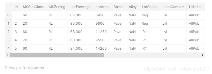
train = pd.read_csv('../input/train.csv')
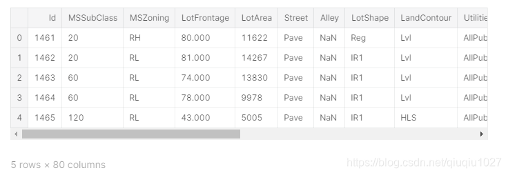
test = pd.read_csv('../input/test.csv')

查看前5行

train.head(5)

test.head(5)

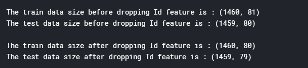
检查样本和特征的数量

#check the numbers of samples and features
print("The train data size before dropping Id feature is : {} ".format(train.shape))
print("The test data size before dropping Id feature is : {} ".format(test.shape))

#Save the 'Id' column
train_ID = train['Id']
test_ID = test['Id']

#Now drop the  'Id' colum since it's unnecessary for  the prediction process.
train.drop("Id", axis = 1, inplace = True)
test.drop("Id", axis = 1, inplace = True)

#check again the data size after dropping the 'Id' variable
print("\nThe train data size after dropping Id feature is : {} ".format(train.shape)) 
print("The test data size after dropping Id feature is : {} ".format(test.shape))

2. 数据处理

异常值

fig, ax = plt.subplots()
ax.scatter(x = train['GrLivArea'], y = train['SalePrice'])
plt.ylabel('SalePrice', fontsize=13)
plt.xlabel('GrLivArea', fontsize=13)
plt.show()

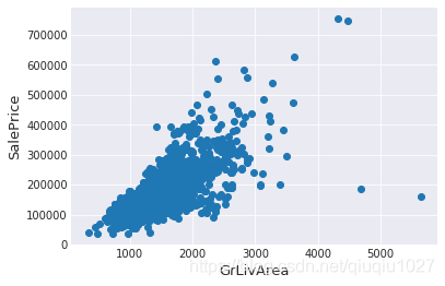
右下角看到两个巨大的grlivrea，价格很低。

#Deleting outliers
train = train.drop(train[(train['GrLivArea']>4000) & (train['SalePrice']<300000)].index)

#Check the graphic again
fig, ax = plt.subplots()
ax.scatter(train['GrLivArea'], train['SalePrice'])
plt.ylabel('SalePrice', fontsize=13)
plt.xlabel('GrLivArea', fontsize=13)
plt.show()

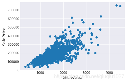
注：

异常值的移除是安全的。我们决定删除这两个，因为它们是非常巨大和非常糟糕的（非常大的面积，非常低的价格）。
训练数据中可能还有其他异常值。但是，如果测试数据中也存在异常值，那么删除所有这些异常值可能会严重影响我们的模型。这就是为什么，我们不把它们全部删除，而只是设法使我们的一些模型在它们上更加健壮。可以参考模型部分。

目标变量
需要预测SalePrice，所以先分析它