tensorflow 入门之五- 多变量线性回归

tensorflow 入门之五- 多变量线性回归

import tensorflow as tf
import matplotlib.pyplot as plt
import numpy as np
tf.__version__

'1.14.0'

# 加载数据
boston=tf.contrib.learn.datasets.load_dataset('boston')
x_train,y_train=boston.data,boston.target
# 预览前五行
x_train[:5],y_train[:5]

(array([[6.3200e-03, 1.8000e+01, 2.3100e+00, 0.0000e+00, 5.3800e-01,
         6.5750e+00, 6.5200e+01, 4.0900e+00, 1.0000e+00, 2.9600e+02,
         1.5300e+01, 3.9690e+02, 4.9800e+00],
        [2.7310e-02, 0.0000e+00, 7.0700e+00, 0.0000e+00, 4.6900e-01,
         6.4210e+00, 7.8900e+01, 4.9671e+00, 2.0000e+00, 2.4200e+02,
         1.7800e+01, 3.9690e+02, 9.1400e+00],
        [2.7290e-02, 0.0000e+00, 7.0700e+00, 0.0000e+00, 4.6900e-01,
         7.1850e+00, 6.1100e+01, 4.9671e+00, 2.0000e+00, 2.4200e+02,
         1.7800e+01, 3.9283e+02, 4.0300e+00],
        [3.2370e-02, 0.0000e+00, 2.1800e+00, 0.0000e+00, 4.5800e-01,
         6.9980e+00, 4.5800e+01, 6.0622e+00, 3.0000e+00, 2.2200e+02,
         1.8700e+01, 3.9463e+02, 2.9400e+00],
        [6.9050e-02, 0.0000e+00, 2.1800e+00, 0.0000e+00, 4.5800e-01,
         7.1470e+00, 5.4200e+01, 6.0622e+00, 3.0000e+00, 2.2200e+02,
         1.8700e+01, 3.9690e+02, 5.3300e+00]]),
 array([24. , 21.6, 34.7, 33.4, 36.2]))

x_train.shape,y_train.shape

((506, 13), (506,))

从上来看, 共有 506 条数据,13 个参数

# 给 x_train 加上首列全为 1 的数据
x_train=np.insert(x_train,0,values=1,axis=1)

x_train.shape

(506, 14)

线性回归模型:
$y=w_0+w_1\ast x1+w_2\ast x_2+w_3\ast x_3+w_4\ast x_4+...+w_n\ast x_n$

也等于
$y=W^T\ast X={\theta }^T\ast X$

# 获取维度
m,n=x_train.shape[0],x_train.shape[1]
m,n

(506, 14)

# 准备 x 和 y. tensorFlow 定义 x,y 用占位符. 
# 对于 x, 需要添加第一列 x0=1, 同时,因为是多维数据,我们需要指定 shape

p_x=tf.placeholder(tf.float32,name="X",shape=[m,n])
p_y=tf.placeholder(tf.float32,name="Y")
p_x,p_y

(<tf.Tensor 'X:0' shape=(506, 14) dtype=float32>,
 <tf.Tensor 'Y:0' shape=<unknown> dtype=float32>)

# 准备 w, 或者 theta
w=tf.Variable(tf.random_normal([n,1]))
w

<tf.Variable 'Variable:0' shape=(14, 1) dtype=float32_ref>

# 定义多元回归模型,tf.matmul 定义矩阵相乘,即"相乘后相加"
y_pre=tf.matmul(p_x,w)
y_pre

<tf.Tensor 'MatMul:0' shape=(506, 1) dtype=float32>

我好奇 tensorflow 是否需要注意矩阵的维度,因此,我们来验证如下,结果发现真的需要注意矩阵的维度:

y_pre=tf.matmul(w,p_x)
y_pre

上诉代码会报错

ValueError: Dimensions must be equal, but are 1 and 506 for 'MatMul_1' (op: 'MatMul') with input shapes: [14,1], [506,14].

误差函数(损失函数)
$cost=(实际值-预测值{)}^2=(y\_pre-y{)}^2$

x = tf.constant([[1., 1.], [2., 2.]])
tf.reduce_mean(x)  # 1.5
tf.reduce_mean(x, 0)  # [1.5, 1.5]
tf.reduce_mean(x, 1)  # [1.,  2.]

# tf.reduce_mean 理解为对一个数组求和
cost=tf.reduce_mean(tf.square(p_y-y_pre,name='cost'))
cost

<tf.Tensor 'Mean:0' shape=() dtype=float32>

计算初始损失值

with tf.Session() as se:
    se.run(tf.global_variables_initializer())
    print(se.run(cost,feed_dict={p_x:x_train,p_y:y_train}))

83079.6

使用优化器优化

# 实例化优化器,最小化 cost. 这里定义计算图, 只定义,不计算
optimizer=tf.train.GradientDescentOptimizer(learning_rate=0.001).minimize(cost)
optimizer

<tf.Operation 'GradientDescent' type=NoOp>

# 记录所有的损失
loses=[]
with tf.Session() as se:
    # 初始化，不然会出错
    se.run(tf.global_variables_initializer())
    for i in range(10):
        # 先执行 optimizer，其 tensorflow 类型为 Option，返回为 None
        # 再执行 cost， 即计算 cost 的值，并返回为第二个值
        # 等价于： run（）先执行 optimizer，参数为 feed_dict 给定的值，
        #          run（）再执行 cost, 参数为 feed_dict
        #          范围值为： （optimizer的返回值，cost 的返回值）
        #          _,lose： 只要第二个值
        _,lose=se.run([optimizer,cost],feed_dict={p_x:x_train,p_y:y_train})
        loses.append(lose)
        print(lose)
        # 这里通过运行 w 来获取其值
#         w_value=se.run(w)

45149.418
3772161300.0
1446208900000000.0
5.6493344e+20
2.2070262e+26
8.6222e+31
inf
inf
inf
inf

上面的 cost 值越来越大，我想应该是我没有将 x 的值进行处理，下面将 x 的值进行处理一下：

$x=\frac{x-mean}{std}=\frac{x-均值}{方差}$

# 将 x 归一化
def mormalize(x):
    mean=np.mean(x)
    std=np.std(x)
    x=(x-mean)/std
    return x

# 记录所有的损失
loses=[]
with tf.Session() as se:
    # 初始化，不然会出错
    se.run(tf.global_variables_initializer())
    for i in range(10000):
        # 先执行 optimizer，其 tensorflow 类型为 Option，返回为 None
        # 再执行 cost， 即计算 cost 的值，并返回为第二个值
        # 等价于： run（）先执行 optimizer，参数为 feed_dict 给定的值，
        #          run（）再执行 cost, 参数为 feed_dict
        #          范围值为： （optimizer的返回值，cost 的返回值）
        #          _,lose： 只要第二个值
        _,lose=se.run([optimizer,cost],feed_dict={p_x:mormalize(x_train),p_y:y_train})
        loses.append(lose)
        # 这里通过运行 w 来获取其值
    w_value=se.run(w)

画出损失函数的图像：从图像得知，其损失值逐渐变小

fig,ax=plt.subplots(figsize=(8,8))
ax.plot(loses)

[<matplotlib.lines.Line2D at 0x22326f1ae88>]

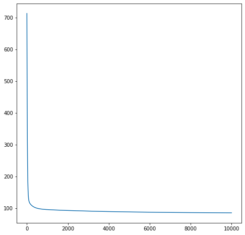
从损失图像上来看，损失基本稳定再 100 左右

# 验证一下数据的维度
w_value,x_train.shape,w_value.shape

(array([[-4.7203207],
        [-4.076027 ],
        [-1.9216492],
        [-3.4172525],
        [-2.949965 ],
        [-3.6158755],
        [-2.8912506],
        [-0.6258089],
        [-4.668212 ],
        [-4.5715165],
        [ 1.1578228],
        [-4.0860596],
        [ 1.6199895],
        [-2.2254002]], dtype=float32), (506, 14), (14, 1))

pre_data=mormalize(x_train)@w_value
pre_data[:3]

array([[22.61672337],
       [22.04721578],
       [22.14444092]])

上面这个就是预测值了,这便完成了预测

画出预测值和实际值的图像来看看

fig,ax=plt.subplots()
ax.plot(y_train)
ax.plot(pre_data,color='r')

[<matplotlib.lines.Line2D at 0x223270df088>]

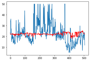
蓝色的是实际的，红色的是预测的，当然，这个模型预测得感觉不靠谱