梯度下降法实现逻辑回归，以及关于为什么 MSE 不能用于分类问题

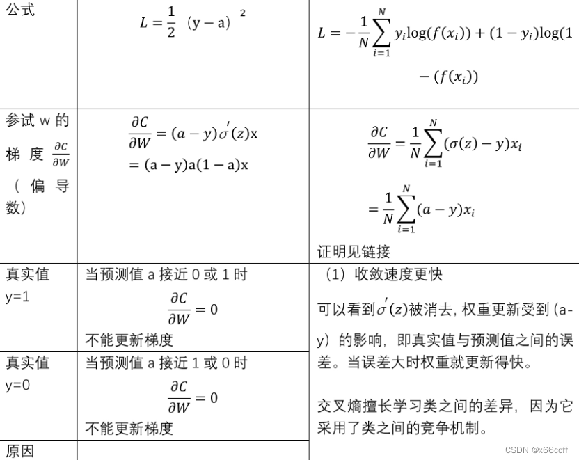
为什么 MSE 不能用于分类

先看这个图，分类在使用交叉熵的时候，$$\frac{dC}{dw}=(a-y)x$$ $$\frac{dC}{db}=(a-y)$$
和线性回归使用 MSE 时候的形式是一样的。
而如果在分类的时候使用MSE，在 $$a=0$$ 或 $$a=1$$ 的时候梯度趋近于0了，因此难以进行更新。

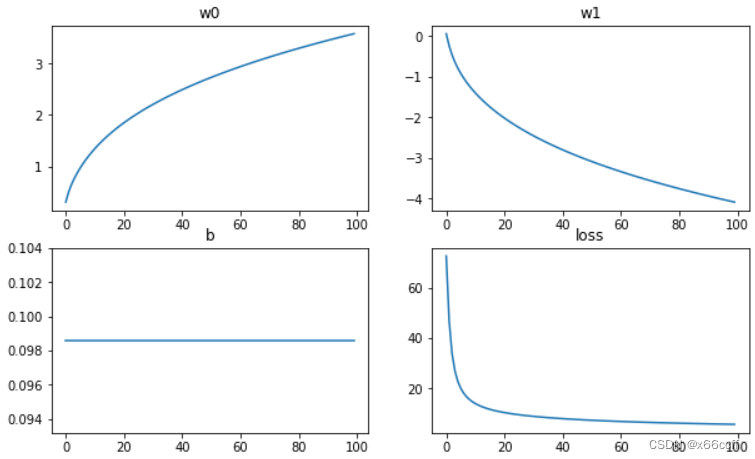
代码

import numpy as np

class logistic_model:
    def __init__(self,dim,lr=0.01):
        self.w = np.random.randn(1,dim)
        self.b = np.random.randn(1)
        self.lr = lr
        self.dim = dim
        self.y_pred = 0

        # y = 1/(1+exp(-wx-b))
    def forward(self,x):
        self.y_pred = 1/(1+np.exp(np.dot(-x,clf.w.T) - self.b))
        return self.y_pred
    

    def backward(self,x,y):
        # C = -(y*log(y_pred)+(1-y)*log(1-y_pred))
        # y_pred = 1/(1+exp(-wx-b))
        
        # dC/dw = x*(y_pred-y)       <---------- 神奇地发现其实 「逻辑回归」在使用交叉熵时，
        # dC/db = (y_pred-y)         <---------- 和 「线性回归」在使用MSE 时的 dC/dw 和 db/dw 的关系是一样的
        
        self.w -= self.lr *  (self.y_pred-y).T @ x 
        self.b -= self.lr * (self.y_pred-y).T @ np.ones(len(x))
    

# cross entropy loss
def loss_cross_entropy(y,y_pred):
    return -np.sum(y*np.log(y_pred))

if __name__ == "__main__":
    
    # generate data
    x = np.random.randn(100,2)
    # generate labels for classification
    y = np.array([[1] if x[i,0] > x[i,1] else [0] for i in range(len(x))])
    
    clf = logistic_model(dim=2,lr=0.01)
    
    epoch = 100
    
    w0_ls = []
    w1_ls = []
    b_ls = []
    loss_ls=[]
    
    for i in range(epoch):
        
        y_pred = clf.forward(x)
        loss = loss_cross_entropy(y, y_pred)
        clf.backward(x,y)
        
        w0_ls.append(clf.w[0][0])
        w1_ls.append(clf.w[0][1])
        b_ls.append(clf.b)
        loss_ls.append(loss)
    
    # plot the loss toghter with weights and biases in subplots with legend
    import matplotlib.pyplot as plt
    plt.figure(figsize=(10,6))
    plt.subplot(221)
    plt.plot(w0_ls)
    plt.title("w0")
    plt.subplot(222)
    plt.plot(w1_ls)
    plt.title("w1")
    plt.subplot(223)
    plt.plot(b_ls)
    plt.title("b")
    plt.subplot(224)
    plt.plot(loss_ls)
    plt.title("loss")
    plt.show()
    
    

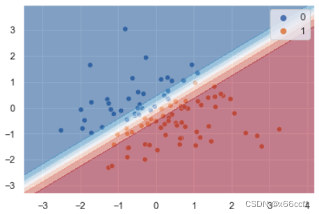
# plot the data and the decision boundary with seaborn
import seaborn as sns
import matplotlib.pyplot as plt
def plot_data(x,y,clf):
    sns.scatterplot(x[:,0],x[:,1],hue=y.flatten())
    x_min,x_max = x[:,0].min()-1,x[:,0].max()+1
    y_min,y_max = x[:,1].min()-1,x[:,1].max()+1
    xx,yy = np.meshgrid(np.arange(x_min,x_max,0.1),np.arange(y_min,y_max,0.1))
    z = clf.forward(np.c_[xx.ravel(),yy.ravel()])
    z = z.reshape(xx.shape)
    plt.contourf(xx,yy,z,cmap="RdBu_r",alpha=0.5)
    plt.show()

plot_data(x, y, clf)