不同插值对比

数据Tb(v)

import numpy as np
import matplotlib.pyplot as plt
import pandas as pd
from scipy.interpolate import interp1d
plt.style.use('https://gitee.com/Astro-Lee/storage/raw/master/mystyle.mplstyle')

info = pd.read_csv('https://gitee.com/Astro-Lee/storage/raw/master/data/Tb(v)_data.csv')
Tb = np.array(info['Tb'])
v = np.array(info['v'])

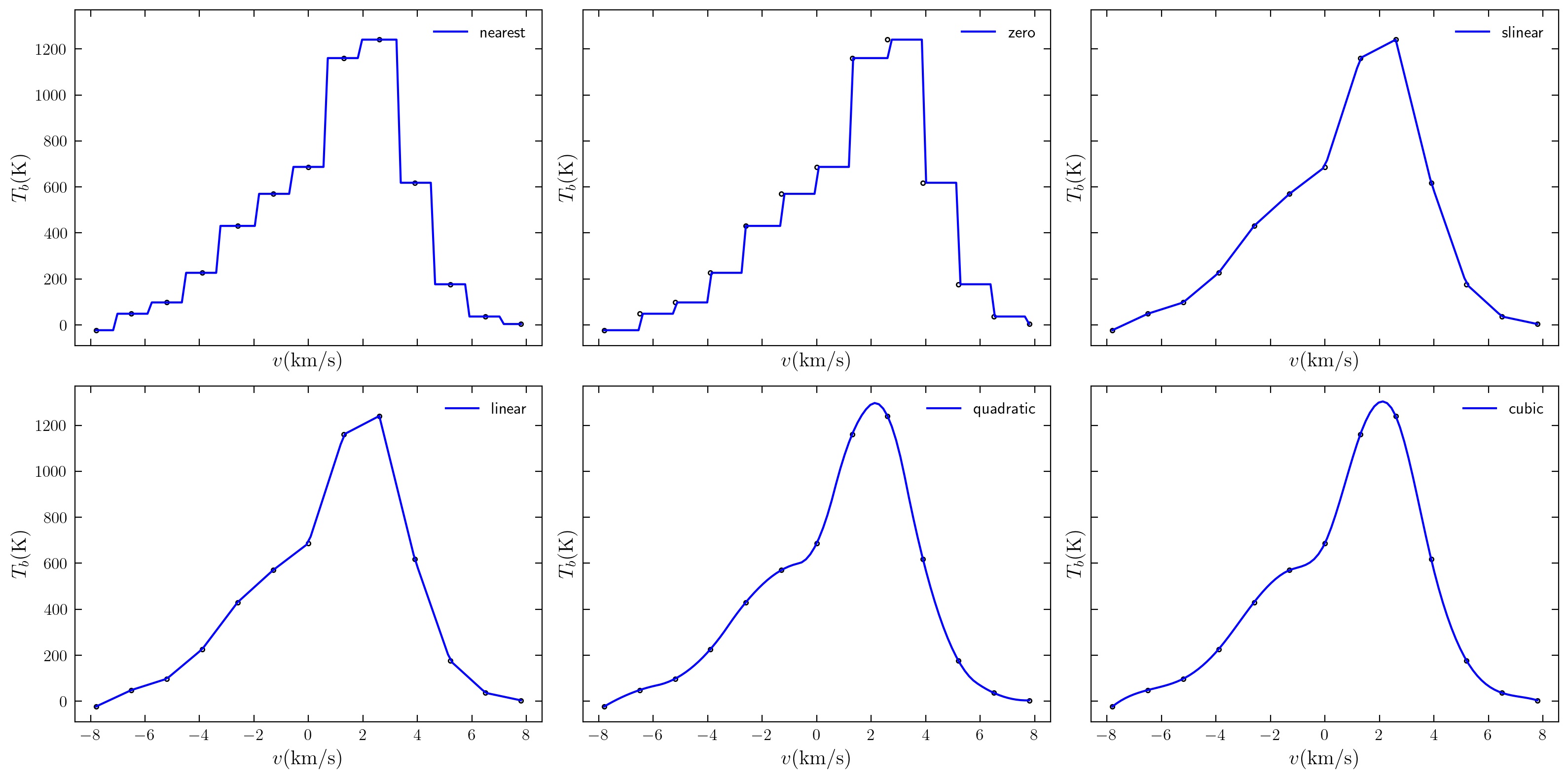
kind = ['nearest','zero','slinear','linear','quadratic','cubic']

u = np.linspace(v[240],v[252],100)
fig = plt.figure(figsize=(16,8),dpi=300)

axes = fig.subplots(2,3,sharex = True,sharey = True)
ax = axes.ravel()

for i,kd in enumerate(kind):
    ax[i].plot(v[240:252+1],Tb[240:252+1],'o',mec='k',mfc='w',ms=3)
    f = interp1d(v[240:252+1],Tb[240:252+1],kind=kd)
    value = f(u)
    ax[i].plot(u,value,'b',label=kd)
    ax[i].legend()
    ax[i].set_xlabel('$v\mathrm{(km/s)}$')
    ax[i].set_ylabel('$T_b\mathrm{(K)}$')
fig.savefig('interp.png')

Gaussian-Legendre integral

#对cubic插值进行积分
from scipy.special import roots_legendre

N = 20                #取样本点个数
a, b = v[240], v[252]   #积分上下限

x, wi = roots_legendre(N)
xi = x*(b-a)/2 + (b+a)/2

s = (b-a)/2 * np.dot(wi, f(xi))
print('积分值:',s)

积分值: 6923.791421843061

Simpson integral

from scipy.integrate import simpson

print('积分值:',simpson(Tb[240:252+1],v[240:252+1]))

积分值: 6883.528256826916