TensorFlow学习笔记（一）之逻辑斯地回归模型及Cifar-10分类的实现

最新推荐文章于 2023-09-03 14:48:54 发布

愤怒的软绵绵

最新推荐文章于 2023-09-03 14:48:54 发布

阅读量1.4k

点赞数 2

分类专栏： Python 数据挖掘文章标签：数据挖掘深度学习 python tensorflow 卷积神经网络

本文链接：https://blog.csdn.net/qq_25742923/article/details/104686812

版权

Python 同时被 2 个专栏收录

18 篇文章 2 订阅

订阅专栏

数据挖掘

6 篇文章 0 订阅

订阅专栏

环境

python 3.6 + TensorFlow 1.13.1 + Jupyter Notebook

介绍

机器学习步骤

数据预处理（采集+去噪）；
模型训练（特征提取+建模）；
模型评估与优化（loss、accuracy及调参）；
模型应用。

深度学习、机器学习、人工智能三者的关系

引自：https://coding.imooc.com/class/259.html

神经网络

神经元是最小的神经网络，以3个神经元为例，结构为：

其表达式为：

$h_{w,b}(x)=f(W^{^{T}}x)=f(\sum_{3}^{i=1}W_{i}x_{i}+b)$
其中， $W^{^{T}}$ 为权重，x为特征，f()为激活函数，b为偏置。

计算举例：

若： $x = [1,2,3];$

$W = [0.1,0.2,0.3];$

$h(W*x) = h(a) = a/10;$

则： $W*x = 1*0.1+2*0.2+3*0.3 = 1.4$

$h(W*x) = h(1.4) = 1.4/10 = 0.14$

二分类逻辑斯地回归模型

引自：https://coding.imooc.com/class/259.html

多分类逻辑斯地回归模型

目标函数（损失函数）

目标函数用于衡量对数据的拟合程度。

主要类型

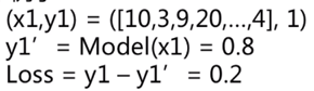
1、二分类：真实值-预测值；

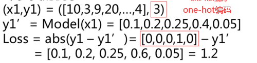
2、多分类：abs(真实值做one-hot编码-预测的概率分布)；

3、平方差损失，表达式为：

$\frac{1}{n}\sum_{x,y}^{ }\frac{1}{2}(y-Model(x))^{2}$

4、交叉熵损失（更适合做多分类的损失函数），表达式为：

$\frac{1}{n}\sum_{x,y}^{ }yln(Model(x))$

注意：多分类在计算目标函数时可以通过one-hot编码实现。

One-hot编码：数值到向量的变换，只有一个位置为1，其他位置均为0。

举例

1、二分类：

2、多分类：

神经网络训练

训练目标

调整参数使得模型在训练集上的损失函数最小。

梯度下降算法

下山算法：找到方向；走一步。引自：https://coding.imooc.com/class/259.html

梯度下降算法与下山算法思想类似：

$\theta =\theta -\frac{\partial L(x,y)}{\partial \theta }$

学习率（步长）： $\alpha$ ，人为设置的，不能过大、过小；

方向： $\frac{\partial L(x,y)}{\partial \theta }$ 。

学习率的影响如下图所示：

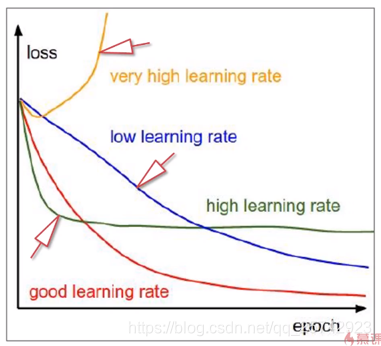
引自：https://coding.imooc.com/class/259.html

TensorFlow实现

计算图模型

命令式编程

声明式编程

先构建图，再填入数据计算。

二者的对比

引自：https://coding.imooc.com/class/259.html

数据处理

下载数据

以CIFAR10为例，下载链接：http://www.cs.toronto.edu/~kriz/cifar.html

准备工作

需要安装包：

在python 2.x中，安装cPickle；

pip install cPickle

在python 3.x中，安装Pickle（建议）；

pip install Pickle

注意：python 3.x也可以用_pickle代替Pickle包（不建议，亲测后面程序报错，不知道是不是这个包的数据导入问题）：

import _pickle as cPickle

读取数据

import os
import numpy as np
import tensorflow as tf
# import _pickle as cPickle
import pickle

cifar_dir = 'dataset/cifar-10-batches-py/'

print(os.listdir(cifar_dir))

运行结果：

查看数据

查看数据结构：

with open(os.path.join(cifar_dir, 'data_batch_1'), 'rb') as f:
    data = cPickle.load(f, encoding='bytes')
    print(type(data))
    
    print(type(data[b'batch_label']))
    print(type(data[b'labels']))
    print(type(data[b'data']))
    print(type(data[b'filenames']))
    print(data[b'data'].shape) # 32 * 32 = 1024 * 3 = 3072
    print(data[b'data'][0:2])
    print(data[b'labels'][0:2])
    print(data[b'batch_label'])
    print(data[b'filenames'][0:2])

运行结果：

查看某一张图：

img_arr = data[b'data'][100]
img_arr = img_arr.reshape((3,32,32))
img_arr = img_arr.transpose((1,2,0))

import matplotlib.pyplot as plt
from matplotlib.pyplot import imshow
%matplotlib inline

imshow(img_arr)

运行结果：

注意：这里需要转换通道，不然图片无法正常显示。

原数据集的每张图的格式为：[32, 32, 3] -> 32 * 32 * 3 = 1024 * 3 = 3072

而我们显示出来的图需要的格式为：[3, 32, 32] -> 3 * 32 * 32 = 3 * 1024 = 3072

数据读取及预处理整体代码

import os
import numpy as np
import tensorflow as tf
# import _pickle as cPickle
import pickle

cifar_dir = 'dataset/cifar-10-batches-py/'
# cifar_dir = 'I:/jupyterWorkDir/testTensorFlow/code/coding-others/cifar-10-batches-py/'

print(os.listdir(cifar_dir))
CIFAR_DIR = cifar_dir



def load_data(filename):
    """read data from data file."""
    with open(filename, 'rb') as f:
        data = pickle.load(f, encoding='bytes')
        return data[b'data'], data[b'labels']

# tensorflow.Dataset.
class CifarData:
    def __init__(self, filenames, need_shuffle):
        all_data = []
        all_labels = []
        for filename in filenames:
            data, labels = load_data(filename)
            all_data.append(data)
            all_labels.append(labels)
        self._data = np.vstack(all_data)
        self._data = self._data / 127.5 - 1
        self._labels = np.hstack(all_labels)
        print(self._data.shape)
        print(self._labels.shape)
        
        self._num_examples = self._data.shape[0]
        self._need_shuffle = need_shuffle
        self._indicator = 0
        if self._need_shuffle:
            self._shuffle_data()
            
    def _shuffle_data(self):
        # [0,1,2,3,4,5] -> [5,3,2,4,0,1]
        p = np.random.permutation(self._num_examples)
        self._data = self._data[p]
        self._labels = self._labels[p]
    
    def next_batch(self, batch_size):
        """return batch_size examples as a batch."""
        end_indicator = self._indicator + batch_size
        if end_indicator > self._num_examples:
            if self._need_shuffle:
                self._shuffle_data()
                self._indicator = 0
                end_indicator = batch_size
            else:
                raise Exception("have no more examples")
        if end_indicator > self._num_examples:
            raise Exception("batch size is larger than all examples")
        batch_data = self._data[self._indicator: end_indicator]
        batch_labels = self._labels[self._indicator: end_indicator]
        self._indicator = end_indicator
        return batch_data, batch_labels

train_filenames = [os.path.join(CIFAR_DIR, 'data_batch_%d' % i) for i in range(1, 6)]
test_filenames = [os.path.join(CIFAR_DIR, 'test_batch')]

train_data = CifarData(train_filenames, True)
test_data = CifarData(test_filenames, False)

构建模型

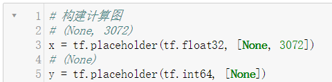
构建计算图

构建x和y，x为输入的数据，y为标签（label），placeholder理解为占位符。

# (None, 3072)
x = tf.placeholder(tf.float32, [None, 3072])
# (None)
y = tf.placeholder(tf.int64, [None])

构建隐含层：

hidden1 = tf.layers.dense(x, 100, activation=tf.nn.relu)
hidden2 = tf.layers.dense(hidden1, 100, activation=tf.nn.relu)
hidden3 = tf.layers.dense(hidden2, 50, activation=tf.nn.relu)

构建w，b和_y，其中w为权重，b为偏置（bias），_y为预测值。

# (3072, 1)
w = tf.get_variable('w', [x.get_shape()[-1], 1],
                   initializer = tf.random_normal_initializer(0,1))
# (1)
b = tf.get_variable('b', [1],
                   initializer = tf.constant_initializer(0.0))
# (None, 3072) * (3072, 1) = (None. 1)
y_ = tf.matmul(x,w) + b

这一步等价于：

y_ = tf.layers.dense(hidden3, 10)

构建预测值的概率分布（p_y_1）和loss（平方差损失）。

# 得到y=1的概率
# (None, 1)
p_y_1 = tf.nn.sigmoid(y_)

# 计算loss (平方差损失)
# (None, 1)
y_reshape = tf.reshape(y, (-1, 1))
y_reshape_float = tf.cast(y_reshape, float32)
loss = tf.reduce_mean(tf.square(y_reshape_float, p_y_1))

这一步等价于：

loss = tf.losses.sparse_softmax_cross_entropy(labels=y, logits=y_)

构建accuracy：

# 计算accuracy
# bool
predict = p_y_1 > 0.5
# bool [0,0,1,1,1,0,1,1,1]
correct_prediction = tf.equal(y_reshape_float, tf.cast(predict, float32))
accuracy = tf.reduce_mean(tf.cast(correct_prediction, float64))

这一步等价于：

# indices
predict = tf.argmax(y_, 1)
# [1,0,1,1,1,0,0,0]
correct_prediction = tf.equal(predict, y)
accuracy = tf.reduce_mean(tf.cast(correct_prediction, tf.float64))

调整learning rate，优化loss：

# (1e-3)是初始化的learning rate
with tf.name_scope('train_op'):
    train_op = tf.train.AdamOptimizer(1e-3).minimize(loss)

构建模型整体代码

# 构建计算图
# (None, 3072)
x = tf.placeholder(tf.float32, [None, 3072])
# (None)
y = tf.placeholder(tf.int64, [None])

hidden1 = tf.layers.dense(x, 100, activation=tf.nn.relu)
hidden2 = tf.layers.dense(hidden1, 100, activation=tf.nn.relu)
hidden3 = tf.layers.dense(hidden2, 50, activation=tf.nn.relu)

'''# (3072, 1)
w = tf.get_variable('w', [x.get_shape()[-1], 1],
                   initializer = tf.random_normal_initializer(0,1))
# (1)
b = tf.get_variable('b', [1],
                   initializer = tf.constant_initializer(0.0))
# (None, 3072) * (3072, 1) = (None. 1)
y_ = tf.matmul(x,w) + b'''
y_ = tf.layers.dense(hidden3, 10)

'''# 得到y=1的概率
# (None, 1)
p_y_1 = tf.nn.sigmoid(y_)

# 计算loss (平方差损失)
# (None, 1)
y_reshape = tf.reshape(y, (-1, 1))
y_reshape_float = tf.cast(y_reshape, float32)
loss = tf.reduce_mean(tf.square(y_reshape_float, p_y_1))'''
loss = tf.losses.sparse_softmax_cross_entropy(labels=y, logits=y_)

'''# 计算accuracy
# bool
predict = p_y_1 > 0.5
# bool [0,0,1,1,1,0,1,1,1]
correct_prediction = tf.equal(y_reshape_float, tf.cast(predict, float32))
accuracy = tf.reduce_mean(tf.cast(correct_prediction, float64))'''
# indices
predict = tf.argmax(y_, 1)
# [1,0,1,1,1,0,0,0]
correct_prediction = tf.equal(predict, y)
accuracy = tf.reduce_mean(tf.cast(correct_prediction, tf.float64))

'''# 梯度下降法优化loss
# (1e-3)是初始化的learning rate
# AdadeltaOptimizer是梯度下降的变种，用于调整learning rate，
# 这是在loss上做，优化最小化的loss值
with tf.name_scope('train_op'):
    train_op = tf.train.AdadeltaOptimizer(1e-3).minimize(loss)'''
with tf.name_scope('train_op'):
    train_op = tf.train.AdamOptimizer(1e-3).minimize(loss)

初始化及运行模型

整体代码

# 初始化
init = tf.global_variables_initializer()
batch_size = 20
train_steps = 100000
test_steps = 100

# run 100k: 50.5%
with tf.Session() as sess:
    sess.run(init)
    for i in range(train_steps):
        batch_data, batch_labels = train_data.next_batch(batch_size)
        loss_val, acc_val, _ = sess.run(
            [loss, accuracy, train_op],
            feed_dict={
                x: batch_data,
                y: batch_labels})
        if (i+1) % 500 == 0:
            print('[Train] Step: %d, loss: %4.5f, acc: %4.5f'
                  % (i+1, loss_val, acc_val))
        if (i+1) % 5000 == 0:
            test_data = CifarData(test_filenames, False)
            all_test_acc_val = []
            for j in range(test_steps):
                test_batch_data, test_batch_labels \
                    = test_data.next_batch(batch_size)
                test_acc_val = sess.run(
                    [accuracy],
                    feed_dict = {
                        x: test_batch_data, 
                        y: test_batch_labels
                    })
                all_test_acc_val.append(test_acc_val)
            test_acc = np.mean(all_test_acc_val)
            print('[Test ] Step: %d, acc: %4.5f'
                  % (i+1, test_acc))

注意事项

1、有时候报莫名其妙的错，建议先检查python版本和运行环境，我之前就是环境运行错了，改错改到怀疑人生，附上代码：

# 查看python版本及运行环境的路径
import sys
print(sys.version)
print(sys.executable)

2、在python 2.x中，读取数据集为：

def load_data(filename):
    """read data from data file."""
    with open(filename, 'rb') as f:
        data = cPickle.load(f)
        return data['data'], data['labels']

在python 3.x中，读取数据集为：

def load_data(filename):
    """read data from data file."""
    with open(filename, 'rb') as f:
        data = pickle.load(f, encoding='bytes')
        return data[b'data'], data[b'labels']

（1）在python 3.x中，如果没有加encoding则会报错：

'ascii' codec can't decode byte 0x8b in position 6: ordinal not in range(128)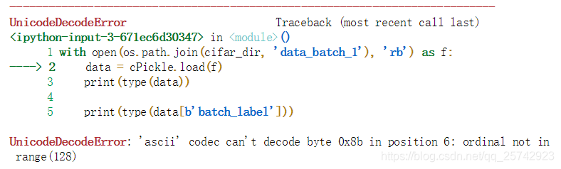

（2）在python 3.x中，data['']如果没有加'b'则会报错：KeyError

参考资料

图片、教程及内容：https://coding.imooc.com/class/259.html

API帮助文档：http://www.tensorfly.cn/tfdoc/api_docs/index.html

愤怒的软绵绵

关注

2
点赞
踩
10

收藏

觉得还不错? 一键收藏
0
评论
TensorFlow学习笔记（一）之逻辑斯地回归模型及Cifar-10分类的实现

环境python 3.6 + TensorFlow 1.13.1 + Jupyter Notebook介绍机器学习步骤数据预处理（采集+去噪）；模型训练（特征提取+建模）；模型评估与优化（loss、accuracy及调参）；模型应用。深度学习、机器学习、人工智能三者的关系引自：https://coding.imooc.com/class/259.html神...
复制链接

扫一扫