How to train Neural Network faster with optimizers?

from:https://towardsdatascience.com/how-to-train-neural-network-faster-with-optimizers-d297730b3713

AsI worked on the last article, I had the opportunity to create my own neural network using only Numpy. It was a very challenging task, but at the same time it significantly broadened my understanding of the processes that take place inside the NN. Among others, this experience made me truly realize how many factors influence neural net’s performance. Selected architecture,proper hyperparameter values or even correct initiation of parameters, are just some of those things... This time however, we will focus on the decision that has a huge impact on learning process speed, as well as the accuracy of obtained predictions — the choice of the optimization strategy. We will look inside many popular optimizers, investigate how they work and compare them with each other.

Note: Due to quite a large range of material that I want to cover, I decided not to include any code snippets in this article. Remember however, that as usual, you can find all the code used to create visualizations on GitHub. I have also prepared a few notebooks that will allow you to better understand the discussed issues.

Optimization of machine learning algorithms

Optimization is a process of searching for parameters that minimize or maximize our functions. When we train machine learning model, we usually use indirect optimization. We choose a certain metric — like accuracy, precision or recall — which indicates how well our model solves a given problem. However, we are optimizing a different cost function J(θ) and hope that minimizing its value will improve metric we care about. Of course, the choice of the cost function is usually related to the specific problem that we aim to tackle. Essentially, it’s deliberately designed to indicate how far from an ideal solution we are. As you can imagine, this topic is quite complicated and is a great topic for a separate article.

Figure 1. Examples of points which are a problem for optimization algorithms.

Traps along the way

Itturns out though, that very often finding a minimum of non-convex cost functions is not easy, and we have to use advanced optimization strategies to locate them. If you have learned differential calculus, you certainly know the concept of local minimum — these are some of the biggest traps that our optimizer can fall into. For those who have not yet come across this wonderful part of the mathematics, I will only say that these are the points where function takes a minimum value, but only in a given region. An example of such a situation is shown on the left hand side of the figure above. We can clearly see that the point located by the optimizer is not the most optimal solution overall.

Overcoming the so-called saddle points is often considered to be even more challenging. These are plateaus, where the value of the cost function is almost constant. This situation is illustrated on the right-hand side of the same figure. At these points the gradient is almost zeroed in all directions making it impossible to escape.

Sometimes, especially in the case of multi-layer networks, we may have to deal with regions where the cost function is very steep. In such places the value of the gradient drastically increases — the exploding gradient — what leads to taking huge steps, often ruining the entire previous optimization. However, this problem can be easily avoided by gradient clipping — defining the maximum allowed gradient value.

Gradient descent

Before we get to know more advanced algorithms, let’s take a look at some of basic strategies. Probably one of the most straightforward approaches is to simply go in direction opposite to the gradient. This strategy can be described by the following equation.

Where α is a hyperparameter called learning rate, which translates into the length of the step that we will take in each iteration. Its selection expresses — in a certain extent — a compromise between the speed of learning and the accuracy of the result that can be obtained. Choosing too small step leads us to tedious calculations and the necessity of performing much more iterations. On the other hand, however, choosing too high value can effectively prevent us from finding the minimum. Such a situation is presented in the Figure 2 — we can see how in subsequent iterations we bounce around, not being able to stabilize. Meanwhile, the model where appropriate step was defined, found at a minimum almost immediately.

Figure 2. Visualization of gradient descent behavior for small and large learning rate values. In order to avoid obscuring the image, only the last ten steps are visible at any time.

In addition, this algorithm is vulnerable to previously described problems of saddle points. Since the size of the correction performed in subsequent iterations is proportional to the calculated gradient, we will not be able to escape from the plateau.

Finally, to top it all off, the algorithm is ineffective — it requires the use of the entire training set in each iteration. This means that in every epoch we have to look at all the examples in order to perform next optimisation step. This may not be a problem when the training set consists of several thousand examples, but as I mentioned in one of my articles — neural networks work best when they have millions of records at their disposal. In that case, it is hard to imagine that in every iteration we use the whole set. It would be a waste of both time and computer memory. All these factors cause that gradient descent, in its purest form, does not work in most cases.

Mini-batch gradient descent

Figure 3. Comparison of gradient descent and mini-batch gradient descent.

Let’s first try to deal with the last of the problems mentioned in the previous chapter — inefficiency. Although vectorization allows us to accelerate calculations, by handling many training examples at once, when the dataset has millions of records the whole process will still take long time to complete.. Let’s try to use a rather trivial solution — divide the whole dataset set into smaller batches and use them for training in subsequent iterations. Our new strategy has been visualised on the animation above. Imagine that the contours drawn on the left symbolize the cost function that we want to optimize. We can see that due to the much smaller amount of data that we need to process, our new algorithm makes decisions much faster. Let’s also pay attention to the contrast in the movement of the compared models. The gradient descent takes rare, relatively large steps with little noise. On the other hand, batch-size gradient descent takes steps more often, but due to the possible diversity in the analyzed data sets, we have much more noise. It is even possible that in one of the iterations we will move in the opposite direction to the intended one. On average, however, we move towards the minimum.

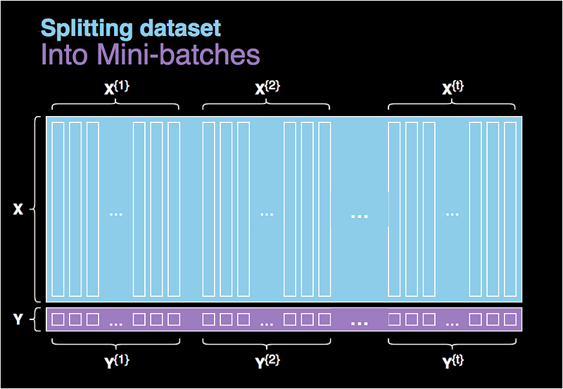
Figure 4. Splitting the dataset into batchs.

I know what you are thinking about…. How to select a batch size? As is often the case in deep learning, the answer is not definitive and depends on the specific case. If the size of our batch is equal to the whole dataset, then we are essentially dealing with an ordinary gradient descent. On the other hand, if the size is 1, then in each iteration we are using only one example from our dataset, as a consequence losing the benefits of vectorisation. This approach is sometimes justified and is called stochastic gradient descent. In reality we usually choose an intermediate value — typically selected from the range of 64 to 512 examples.

Exponentially weighted averages

This idea is used in many areas such as statistics, economics and even deep learning. Many advanced NN optimization algorithms use this concept, because it allows us to continue optimization even if the gradient calculated at the given point is zero. Let’s take a few moments to understand this algorithm. As an example we will use the share value of the biggest tech company from the last year.

Figure 5. Visualization showing Exponentially weighted averages calculated for different β values.

EWA is essentially about averaging many previous values in order to become independent of local fluctuations and focus on the overall trend. It’s value is calculated using recursive formula shown above, where β is the parameter used to control the range of values to be averaged. We can say that in subsequent iterations we taken into account 1/(1 - β) examples. For large values of β the graph we get is much smoother, because we average many records. On the other hand, our chart moves more and more to the right, because when we average over a large period of time, the EWA adapts more slowly to the new trend. This can be seen in Figure 5, where we illustrated the actual value of shares at closing as well as 4 graphs showing the value of exponentially weighted averages calculated for different beta parameters.

Gradient descent with momentum

This strategy leverages exponentially weighted averages to avoid troubles with points where gradient of cost functions is close to zero. In simple words, we allow our algorithm to gain momentum, so that even if the local gradient is zero, we still move forward relying on the previously calculated values. For this reason, it is almost always a better choice than a pure gradient descent.

As usual we use back propagation, to calculate the value of dW and db for each layer of our network. This time however, instead of directly using the calculated gradient to update the values of our NN parameters, we first calculate the intermediate values of VdW and Vdb. These values are in fact EWA of derivatives of the cost function in respect of individual parameters. Finally, we will use VdW and Vdb in gradient descent. The whole process can be described with following equations. It is also worth noting that the implementation of this method requires to store EWA values between iterations. You can see the details in one of the notebooks on my repository.

Figure 6. Gradient descent with momentum.

Let’s now try to develop a certain intuition about the influence of EWA on the behaviour of our model. Once again, let’s imagine that the contours drawn below symbolize the cost function that we optimize. The visualization above shows a comparison between standard gradient descent and GD with momentum. We can see that the shape of the graph of the cost function forces a very slow way of optimization. As in the example of stock market prices, the use of exponentially weighted averages allows us to focus on the leading trend instead of the noise. Component indicating minimum is amplified and component responsible for the oscillations is slowly eliminated. What’s more, if we obtain gradients pointing a similar direction in subsequent updates, the learning rate will increase. This leads to faster convergence and reduced oscillations. This method, however, has a disadvantage — as you approach the minimum, the momentum value increases and may become so large that the algorithm will not be able to stop at the right place.

RMSProp

Another way to improve the performance of gradient descent is to apply the RMSProp strategy — Root Mean Squared Propagation — which is one of the most frequently used optimizers. This is another algorithm that uses exponentially weighted averages. Moreover, it is adaptive — it allows for individual adjustment of the learning rate for each parameter of the model. Subsequent parameter values are based on previous gradient values calculated for particular parameter.

Using the example from Figure 6. and the equations above, let us consider the logic behind this strategy. According to the name, in each iteration we calculate element-wise squares of derivates of the cost function in respect of the corresponding parameters. In addition, we use EWA to average the values obtained in recent iterations. Finally, before we update the values of our network parameters, the corresponding gradient components are divided by the square root of the sum of squares. This means that the learning rate is reduced faster for parameters where the gradient is large and slower for parameters where the gradient is small. In this way, our algorithm reduces oscillations and prevents noise them from dominating the signal. In order to avoid dividing by zero (numerical stability), we also add to the denominator a very small value, marked in referred formulas as ɛ.

I must admit that while writing this article I had two wow-moments — moments when I was really shocked by the quality leap between the optimizers I analysed. The first one was when I saw the difference in training time between standard gradient descent and mini-batch. The second now, when I compared the RMSprop with everything we have seen so far. However, this method has its drawbacks. As the denominator of the above equations increases in each iteration, our learning rate is getting smaller. As a consequence, this may cause our model to stop completely.

Figure 7. Optimizers comparison.

Adam

Last but not least, let me tell you about Adaptive Moment Estimation. It is an algorithm which, like RMSProp, works well in a wide range of applications. It takes advantage of the biggest pros of RMSProp, and combine them with ideas known from momentum optimization. The result is a strategy that allows for quick and effective optimization. The above figure shows how well discussed optimizers handle optimization of a difficult part of the function. You can immediately see that Adam is doing very well in this case.

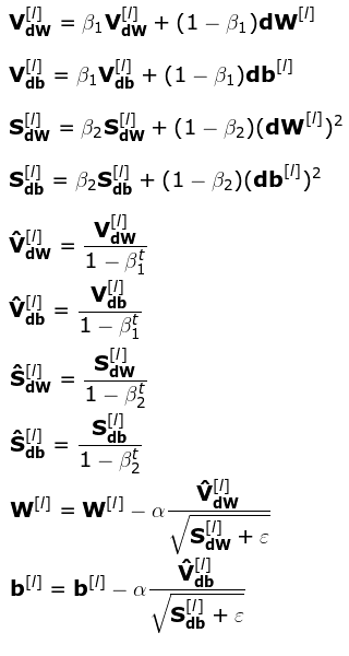
Unfortunately, as the effectiveness of our method increases, the complexity of calculations grows as well. It’s true…. Above, I have written ten matrix equations that describe single iteration of optimization process . I know from experience that some of you — especially those less familiar with mathematicians — will now be in a grave mood. Don’t worry! Note that there is nothing new there. These are the same equations that were previously written for momentum and RMSProp optimizers. This time we will simply use both ideas at once.

Conclusion

Ihope that I have managed to explain these difficult issues in a transparent way. Work on this post allowed me to grasp how important it is to choose the right optimizer. Understanding of these algorithms allows to use them consciously, Understanding how changes in individual hyperparameters affect the performance of the whole model.

Congratulations if you managed to get here. It was certainly not the easiest reading. If you like this article follow me on Twitter and Medium and see other projects I’m working on, on GitHub and Kaggle. This article is the fourth part of the “Mysteries of Neural Networks” series, if you haven’t had the opportunity yet, read the other articles. And if you have interesting ideas for the next posts, write in the comments. Stay curious!