


摘要:本文简单叙述了如何根据标准普尔500指数使用线性回归来预测股票的走势
本文内容来源:https://www.dataquest.io/mission/58/regression-basics
标准普尔500(S&P 500)说明:http://www.investopedia.com/ask/answers/05/sp500calculation.asp
转载自:http://www.cnblogs.com/kylinlin/p/5295254.html
原始数据展现(使用了2005年至2015年的数据)
import pandas
sp500 = pandas.read_csv("sp500.csv")
注意到上面的数据中有一些行(如第六行)的value值为点号(.),这是因为这个日期在美国是一个假日,所以没有股票交易信息,现在要过滤掉这些行
sp500 = sp500[sp500['value'] != '.']格式化数据
为了更容易地使用机器学习的算法,需要把用来预测的值和预测后的真实值放在同一行,在这个例子中,我们要根据每一天的股票指数来预测下一个交易日的股票指数,所以要在每一行上增加下一天指数的列,我们需要的是这样格式的数据

next_day = sp500["value"].iloc[1:]
sp500 = sp500.iloc[:-1,:] # 去掉最后一行
sp500["next_day"] = next_day.values
在导入文件的时候,Pandas会自动为每一列的数据推断数据格式,但由于在导入原始的文件时有一些行(如第六行)的value值为点号(.),所以pandas把该列认为是字符类型,而不是float类型,需要将该列转换数据格式
# 原始的数据格式
print(sp500.dtypes)
sp500['value'] = sp500['value'].astype(float)
sp500['next_day'] = sp500['next_day'].astype(float)
# 转换后的数据格式
print(sp500.dtypes)
建立模型
使用sckit-learn包中的线性回归(http://scikit-learn.org/stable/modules/generated/sklearn.linear_model.LinearRegression.html#sklearn.linear_model.LinearRegression)来预测下一个交易日的股票指数
#导入类

from sklearn.linear_model import LinearRegression

# 初始化

regressor = LinearRegression()

# predictors变量需要是一个dataframe,而不能是一个series

predictors = sp500[["value"]] # 这是一个dataframe

to_predict = sp500["next_day"] # 这是一个series

# 训练这个线性回归模型

regressor.fit(predictors, to_predict)

# 根据模型生成预测值

next_day_predictions = regressor.predict(predictors)

print(next_day_predictions)
评估模型
一个经常用于评估回归模型的指标是均方差(mean squared error, MSE),计算公式:

mse = sum((to_predict - next_day_predictions) ** 2) / len(next_day_predictions)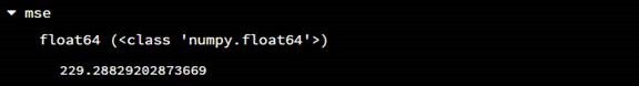
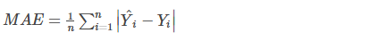
另外两个常用的指标是根均方差(root mean squared error, RMSE)和平均绝对误差(mean absolute error, MAE)
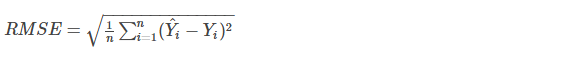
import math
rmse = math.sqrt(sum((predictions - test["next_day"]) ** 2) / len(predictions))
mae = sum(abs(predictions - test["next_day"])) / len(predictions)
在上面的评估模型中存在一个巨大的错误,那就是过度拟合:使用了同样的数据来训练模型和进行预测。想象一下,你告诉他人 2 + 2 等于4,然后问他2 + 2的结果,他可以马上回答你正确的答案,但是他未必明白加法运算的原理,假如你问他3 + 3的结果,他就可能回答不了。同样地,你用一批数据来训练这个回归模型,然后再用同样的数据来进行预测,会造成一个结果,那就是错误率非常低,因为这个模型早就知道了每个正确的值。
用来避免过度拟合的最好方法就是将训练的数据和用来预测(测试)的数据分开
import numpy as np
import random
np.random.seed(1)
random.seed(1)
#将sp500进行随机重排
sp500 = sp500.loc[np.random.permutation(sp500.index)]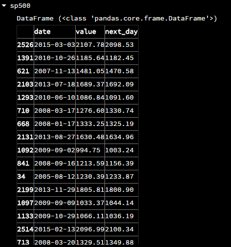
# 选择前70%的数据作为训练数据
highest_train_row = int(sp500.shape[0] * .7)
train = sp500.loc[:highest_train_row,:]
#选择后30%的数据作为测试数据
test = sp500.loc[highest_train_row:,:]
regressor = LinearRegression()
predictors = train[['value']]
to_predict = train['next_day']
regressor.fit(predictors, to_predict)
next_day_predictions = regressor.predict(test[['value']])
mse = sum((next_day_predictions - test['next_day']) ** 2) / len(next_day_predictions)
数据可视化
除了上面用来评估模型误差的指标可以说明一个模型的正确性,也可以使用图表来展现,下面做一个散点图,很坐标为测试数据的value列,纵坐标为测试数据的next_day列。然后在上面再做一个折线图,横坐标同样为测试数据的value列,纵坐标为使用模型预测后的结果
import matplotlib.pyplot as plt
plt.scatter(test['value'], test['next_day'])
plt.plot(test['value'], predictions)
plt.show()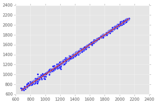


 1518
1518

 被折叠的 条评论
为什么被折叠?
被折叠的 条评论
为什么被折叠?
 到【灌水乐园】发言


