自制深度学习推理框架-第十一节-再探Tensor类并构建计算图的图关系

自制深度学习推理框架-第十一节-再探Tensor类并准备算子的输入输出

本课程介绍

我写了一个《从零自制深度学习推理框架》的课程，课程语言是 C++，课程主要讲解包括算子实现和框架设计的思路，国内算是独一份，目前已登上 HelloGithub 最新一期。我这个仓库算是课程的上游项目，根据上游项目来规划课程内容。

b 站视频链接: https://space.bilibili.com/1822828582

github 链接: https://github.com/zjhellofss/KuiperInfer 欢迎点赞和 PR 已经发布 Docker

本节课代码

git clone  https://github.com/zjhellofss/KuiperCourse
git checkout ten

再探张量类Tensor

自从我们第二节讲完Tensor之后，再也没有好好地看过Tensor这个重要的数据结构。如同本课程第二节所言，Tensor表示的是一个多维向量，用于存储模型的输入、输出以及各层权重等数据。

因此在第二节中我们编写的Tensor类其实并不能满足我们的使用需要，我们将在这一节以代码阅读的方式来看看一个完全版本的Tensor应该具备怎样的要素，同时我们对Tensor类的分析来看看在C++中一个设计好的类应该是怎么样的。

Tensor<float>::Tensor(uint32_t channels, uint32_t rows, uint32_t cols) {
  data_ = arma::fcube(rows, cols, channels);
  if (channels == 1 && rows == 1) {
    this->raw_shapes_ = std::vector<uint32_t>{cols};
  } else if (channels == 1) {
    this->raw_shapes_ = std::vector<uint32_t>{rows, cols};
  } else {
    this->raw_shapes_ = std::vector<uint32_t>{channels, rows, cols};
  }
}

在这里，raw_shape记录的是另外一个方面的形状信息，主要用于review和flatten层中。

举一个简单的例子，当Tensor将一个大小为(2,16,1)的Tensor reshape到(32,1,1)的大小时，raw_shapes变量会被记录成(32). 将一个大小为(2,16, 2)的Tensor reshape到(2, 64)的大小时，raw_shapes会被记录成(2,64).

那这样做的目的是什么呢？原来的Tensor不能在逻辑上区分当前的张量是三维的、二维的还是一维的，因为实际的数据存储类arma::fcube总是一个三维数据。

Tensor中的逻辑维度

我们通过raw_shapes来记录当前的实际维度，当raw_shapes的长度为2时，说明当前的张量是二维的。当raw_shapes的长度为1的时候，说明当前的张量是一维的。

这样一来，系统中就有两种类型的shape, 第一种shape是数据本身的维度，例如有一个大小为(32,1,1)的data，它的shapes就会是32x32x1, 但是对于raw_shapes这个数据对应的维度就是(32, )，这样一来，我们就可以在后续的推理知道data的逻辑维度是多少(现在是一个一维的张量).

列优先的Reshape

void Tensor<float>::ReRawshape(const std::vector<uint32_t>& shapes) {
  CHECK(!this->data_.empty());
  CHECK(!shapes.empty());
  const uint32_t origin_size = this->size();
  uint32_t current_size = 1;
  for (uint32_t s : shapes) {
    current_size *= s;
  }
  CHECK(shapes.size() <= 3);
  CHECK(current_size == origin_size);

  if (shapes.size() == 3) {
    this->data_.reshape(shapes.at(1), shapes.at(2), shapes.at(0));
    this->raw_shapes_ = {shapes.at(0), shapes.at(1), shapes.at(2)};
  } else if (shapes.size() == 2) {
    this->data_.reshape(shapes.at(0), shapes.at(1), 1);
    this->raw_shapes_ = {shapes.at(0), shapes.at(1)};
  } else {
    this->data_.reshape(shapes.at(0), 1, 1);
    this->raw_shapes_ = {shapes.at(0)};
  }
}

我们再来分析一下这个函数，如果传入的shapes是1维的，就相当于将数据展开为(elem_size,1,1)，并将逻辑维度赋值为1. 如果传入的shapes，相当于将数据展开为(shapes.at(0), shapes.at(1), 1). 我们来看看下面的这个图例：

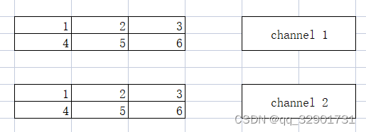
它的大小是channel = 2, rows = 2, cols = 3，当前的raw_shapes等于(2,2,3) 如果将这个tensor调整到到一维的，那么就如下图所示：

当前的rawshapes等于(12)，我们也就可以通过判断rawshapes的方式来得知当前的逻辑维度。我们可以看到Reshape的方式是列优先的，这是因为负责管理数据的armadillo::cube是一个列优先的容器。

行优先的Reshape

那如果我们在某些情况下需要行优先的Reshape呢？

void Tensor<float>::ReView(const std::vector<uint32_t>& shapes) {
  CHECK(!this->data_.empty());
  const uint32_t target_channels = shapes.at(0);
  const uint32_t target_rows = shapes.at(1);
  const uint32_t target_cols = shapes.at(2);
  arma::fcube new_data(target_rows, target_cols, target_channels);

  const uint32_t plane_size = target_rows * target_cols;
  for (uint32_t c = 0; c < this->data_.n_slices; ++c) {
    const arma::fmat& channel = this->data_.slice(c);
    for (uint32_t c_ = 0; c_ < this->data_.n_cols; ++c_) {
      const float* colptr = channel.colptr(c_);
      for (uint32_t r = 0; r < this->data_.n_rows; ++r) {
        const uint32_t pos_index =
            c * data_.n_rows * data_.n_cols + r * data_.n_cols + c_;
        const uint32_t ch = pos_index / plane_size;
        const uint32_t row = (pos_index - ch * plane_size) / target_cols;
        const uint32_t col = (pos_index - ch * plane_size - row * target_cols);
        new_data.at(row, col, ch) = *(colptr + r);
      }
    }
  }
  this->data_ = new_data;
}

我们只能通过位置计算的方式来对逐个元素进行搬运， const uint32_t plane_size = target_rows * target_cols;来计算行数和列数相乘的积。

const uint32_t pos_index = c * data_.n_rows * data_.n_cols + r * data_.n_cols + c_; 得 到调整前的元素下标，随后我们计算调整后的通道下标位置：ch = pos_index / plane_size，同理计算row,col等调整位置后的行、列坐标。

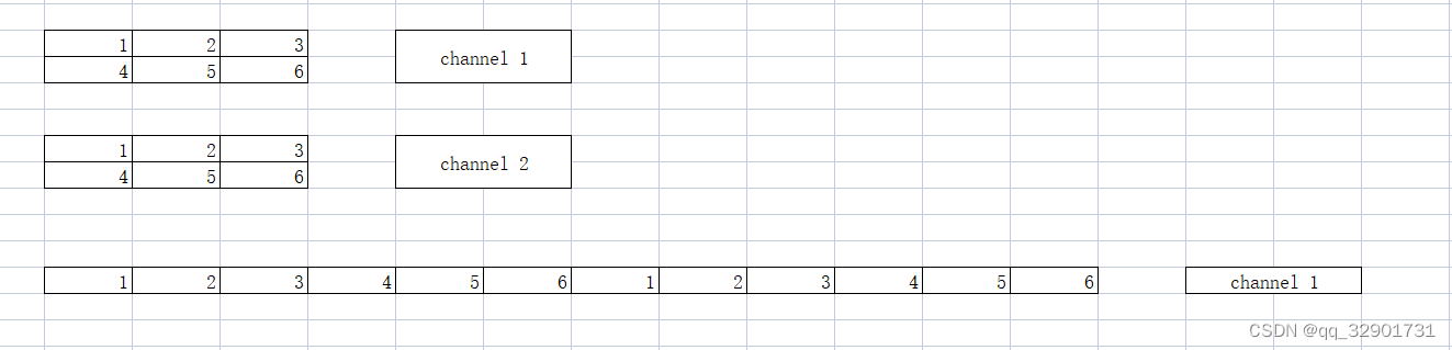
可以通过图例看到原本的张量按照行优先的顺序完成了展开。

其他的辅助方法

TensorElementMultiply用于对两个张量逐点相乘，TensorElementAdd用于两个张量的相加，这类方法不做赘述，见名思意。

构建计算图关系

内容回顾

我们在回顾一下之前的内容，我们根据pnnx计算图得到了我们的计算图，我们的计算图由两部分组成，分别是kuiper_infer::RuntimeOperator和kuier_infer::RuntimeOperand.

但是作为一个计算图，计算节点之间往往是有连接的，包括从input operator到第一个计算节点再到第二个计算节点，直到最后的输出节点output operator，我们再来回顾一下这两个数据结构的具体定义：

struct RuntimeOperator {
  int32_t meet_num = 0; /// 计算节点被相连接节点访问到的次数
  ~RuntimeOperator() {
    for (auto &param : this->params) {
      if (param.second != nullptr) {
        delete param.second;
        param.second = nullptr;
      }
    }
  }
  std::string name; /// 计算节点的名称
  std::string type; /// 计算节点的类型
  std::shared_ptr<Layer> layer; /// 节点对应的计算Layer

  std::vector<std::string> output_names; /// 节点的输出节点名称
  std::shared_ptr<RuntimeOperand> output_operands; /// 节点的输出操作数

  std::map<std::string, std::shared_ptr<RuntimeOperand>> input_operands; /// 节点的输入操作数
  std::vector<std::shared_ptr<RuntimeOperand>> input_operands_seq; /// 节点的输入操作数，顺序排列
  std::map<std::string, std::shared_ptr<RuntimeOperator>> output_operators; /// 输出节点的名字和节点对应

  std::map<std::string, RuntimeParameter *> params;  /// 算子的参数信息
  std::map<std::string, std::shared_ptr<RuntimeAttribute> > attribute; /// 算子的属性信息，内含权重信息
};

1. std::map<std::string, std::shared_ptr> output_operators;
   我们重点来看这个定义，它是当前这个计算节点的下一个计算节点，当数据在当前RuntimeOperator上计算完成之后，系统会读取output_operators中准备就绪的算子并开始执行。
2. std::map<std::string, std::shared_ptr> input_operands; 是当前计算节点所需要的输入，它往往来自于上一个RuntimeOperator的输入。
3. std::shared_ptr output_operands; 是当前节点计算得到的输出，它是通过当前的op计算得到的。

具体的流程是这样的，假设我们在系统中有三个RuntimeOperators，分别为op1,op2和op3. 这三个算子的顺序是依次执行的，分别是op1–>op2–>op3.

• 当我们执行第一个算子op1的时候，需要将来自于图像的输入填充到op1->input_operands中。
• 第一个算子op1开始执行，执行的过程中读取op1->input_operands并计算得到相关的输出，放入到op1->output_operands中
• 从op1的output_operators中读取到ready的op2
• 第二个算子op2开始执行，执行的过程读取op1->output_operands并拷贝op2->input_operands中，随后op2算子开始执行并计算得到相关的输出，放入到op2->output_operands中。

怎么构建图关系

图关系的构建流程放在RunGraph::Init中：

  // 构建图关系
  for (const auto &current_op : this->operators_) {
    const std::vector<std::string> &output_names = current_op->output_names;
    for (const auto &next_op : this->operators_) {
      if (next_op == current_op) {
        continue;
      }
      if (std::find(output_names.begin(), output_names.end(), next_op->name) !=
          output_names.end()) {
        current_op->output_operators.insert({next_op->name, next_op});
      }
    }
  }

• const std::vector<std::string> &output_names = current_op->output_names; 存放的是当前op的output_names，output_names也就是当前算子的后一层算子的名字。对于op1，它的output_names就是op2的name.
• const auto &next_op : this->operators_ 我们遍历整个图中的RuntimeOperators，如果遇到next_op的name和当前current_op->output_name是一致的，那么我们就可以认为next_op是当前op的下一个节点之一。
• current_op->output_operators.insert({next_op->name, next_op}); 将next_op插入到current_op的下一个节点当中。
• 这样一来，当current_op执行完成之后就取出next_op，并将当前current_op的输出output_opends（输出）拷贝到next_op的input_operands（输入）中。

找到op list(this->operators)中的输入和输出节点

总所周知，一个图一定有一个输入和输出（图的执行好像在走迷宫，就好像我们走迷宫之前需要先指定迷宫的输入输出位置）

所以我们首先要找到计算图中的输入和输出节点：

  this->input_operators_maps_.clear();
  this->output_operators_maps_.clear();

  for (const auto &kOperator : this->operators_) {
    if (kOperator->type == "pnnx.Input") {
      this->input_operators_maps_.insert({kOperator->name, kOperator});
    } else if (kOperator->type == "pnnx.Output") {
      if (kOperator->name == output_name) {
        this->output_operators_maps_.insert({kOperator->name, kOperator});
      } else {
        LOG(FATAL) << "The graph has two output operator!";
      }
    } else {
      std::shared_ptr<Layer> layer = RuntimeGraph::CreateLayer(kOperator);
      CHECK(layer != nullptr) << "Layer create failed!";
      if (layer) {
        kOperator->layer = layer;
      }
    }
  }

• kOperator->type == “pnnx.Output” 找到this->operators中的输出节点，但是目前Kuiperinfer只支持一个输出节点，其实也可以多输出，作为一个教学框架我实在不想支持这种corner case
• 同理: kOperator->type == “pnnx.Input” 来找到图中，也就是op list中的输入节点

初始化各算子的输入和输出空间

我们知道除了一整个图有输入输出，每个RuntimeOperator也有对应的输入输出，对应在结构中就是：

struct RuntimeOperator {
	...
	...
   std::map<std::string, std::shared_ptr<RuntimeOperand>> input_operands; /// 节点的输入操作数
   std::shared_ptr<RuntimeOperand> output_operands; /// 节点的输出操作数

为什么这里的input_operand是一个maps呢，这一点我们在计算图中讲过，因为一个operetor的输入可能来自于多个其他operator, 比如说add operator.

无论是Operator的输入还是输出，都是由RuntimeOprand来存储的，RuntimeOperand的结构为：

struct RuntimeOperand {
  std::string name;                                     /// 操作数的名称
  std::vector<int32_t> shapes;                          /// 操作数的形状
  std::vector<std::shared_ptr<Tensor<float>>> datas;    /// 存储操作数
  RuntimeDataType type = RuntimeDataType::kTypeUnknown; /// 操作数的类型，一般是float
};

可以看到这里的RuntimeOperand::datas就是存储具体数据的地方，我们初始化输入输出的空间也就是要在推理之前先根据shapes来初始化好这里datas的空间，初始化的过程放在如下的两个函数中：

  RuntimeGraphShape::InitOperatorInputTensor(operators_);
  RuntimeGraphShape::InitOperatorOutputTensor(graph_->ops, operators_);

初始化输入

代码位于runtime_ir.cpp的InitOperatorInputTensor中
RuntimeGraphShape::InitOperatorInputTensor(operators_) 这个函数的输入是operator list, 所以将在这个函数中对所有的op进行输入和输出空间的初始化。

• 得到一个op的输入空间input_operands

     const std::map<std::string, std::shared_ptr<RuntimeOperand>> &
      		input_operands_map = op->input_operands;

• 得到input_operands中记录的数据应有大小input_operand_shape和存储数据的变量input_datas

auto &input_datas = input_operand->datas;

CHECK(!input_operand_shape.empty());
const int32_t batch = input_operand_shape.at(0);
CHECK(batch >= 0) << "Dynamic batch size is not supported!";
CHECK(input_operand_shape.size() == 2 ||
      input_operand_shape.size() == 4 ||
      input_operand_shape.size() == 3)

• 我们需要根据input_operand_shape中记录的大小去初始化input_datas. 而input_operand_shape可能是三维的，二维的以及一维的，如下方所示

1. input_operand_shape : (batch, elemsize) 一维的
2. input_operand_shape : (batch, rows,cols) 二维的
3. input_operand_shape : (batch, rows,cols, channels) 三维的

如果当前input_operand_shape是二维的数据，也就是说输入维度是(batch,rows,cols)的. 我们首先对batch进行遍历，对一个batch的中的数据input_datas= op->input_operand(输入)进行初始化。

input_datas.resize(batch);
for (int32_t i = 0; i < batch; ++i) {
}

在for循环内，它会调用如下的方法去初始化一个二维的张量：

input_datas.at(i) = std::make_shared<Tensor<float>>(1, input_operand_shape.at(1), input_operand_shape.at(2));

这就和我们上面的课程内容对应上了，Tensor<float>原本是一个三维数据，我们怎么在逻辑上给他表现成一个二维的张量呢？这就要用到我们上面说到的raw_shapes了。

Tensor<float>::Tensor(uint32_t channels, uint32_t rows, uint32_t cols) {
  data_ = arma::fcube(rows, cols, channels);
  if (channels == 1 && rows == 1) {
    this->raw_shapes_ = std::vector<uint32_t>{cols};
  } else if (channels == 1) {
    this->raw_shapes_ = std::vector<uint32_t>{rows, cols};
  } else {
    this->raw_shapes_ = std::vector<uint32_t>{channels, rows, cols};
  }
}

Tensor的初始化函数通过传入的参数来确定raw_shapes的维度

• 当传入(1, input_operand_shape.at(1), input_operand_shape.at(2))时候，我们会将raw_shapes的维度定义成两维，也就是channels = 1这种情况。

• 调用并初始化一维的数据也同理, 在初始化的过程中会调用(channels1&&rows1) 这个条件判断，并将raw_shapes这个维度定义成一维。

input_datas.at(i) = std::make_shared<Tensor<float>>(1, input_operand_shape.at(1), 1)

避免第二次的初始化

我们在如上的过程中，完成了对operator->input_operands的初始化，也就是完成了operator->input_operands->datas的初始化。

所以，我们在第二次调用这个函数的时候不需要再对input_data进行初始化了，只需要检查参数是否正确即可，如下所示：

Tips: 我们input_data.at(i)的大小是根据input_operand.input_shapes来确定的，所以在以后校验的时候只需要确定input_data的维度和input_operand.input_shapes一致就可以了

          for (int32_t i = 0; i < batch; ++i) {
            const std::vector<uint32_t> &input_data_shape =
                input_datas.at(i)->shapes();
            CHECK(input_data_shape.size() == 3)
                    << "The origin shape size of operator input data do not equals "
                       "to three";
            if (input_operand_shape.size() == 4) {
              CHECK(input_data_shape.at(0) == input_operand_shape.at(1) &&
                  input_data_shape.at(1) == input_operand_shape.at(2) &&
                  input_data_shape.at(2) == input_operand_shape.at(3));
            } else if (input_operand_shape.size() == 2) {
              CHECK(input_data_shape.at(1) == input_operand_shape.at(1) &&
                  input_data_shape.at(0) == 1 && input_data_shape.at(2) == 1);
            } else {
              // current shape size = 3
              CHECK(input_data_shape.at(1) == input_operand_shape.at(1) &&
                  input_data_shape.at(0) == 1 &&
                  input_data_shape.at(2) == input_operand_shape.at(2));
            }
          }

实验部分

实验部分请按clone仓库后,checkout到ten 分支. 具体的操作请看视频