用NumPy向量化python实现AODE半朴素贝叶斯分类器——以西瓜书第七章习题7.6为例

一、发文起因：

        1、为一起学习机器学习的同伴提供参考

        2、求大佬看看处理思路有没有问题

二、程序亮点：

        1、采用Numpy向量化进行计算，提高了计算速度

        2、对连续型数据进行了针对性的处理

三、输入数据结构：

        AODE类输入数据遵循以下结构：

                1、数据集纵向排列，每一行是一组数据参数

                2、标签应置于数据组的最后一列

                3、以np.array（[]）格式进行输入shape=（a，d+1）a为数据量，d为参数个数

        大家可根据此结构直接套用主代码。ps：使用前务必阅读注释

        其余参数参照主代码和注释。

四、源码

（本人非计算机类、数学类专业，不足之处敬请指出）

import numpy as np
import matplotlib.pyplot as plt
import math
from scipy.stats import multivariate_normal

def load_data():#载入数据，此处载入数据的函数是搬运过来的与AOME_mode所要求的数据结构有出入，在主程序中对数据结构进行再处理
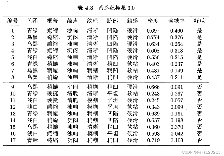
    features = np.array([
        [1, 2, 2, 1, 0, 1, 2, 2, 2, 1, 0, 0, 1, 0, 2, 0, 1],
        [2, 2, 2, 2, 2, 1, 1, 1, 1, 0, 0, 2, 1, 1, 1, 2, 2],
        [1, 0, 1, 0, 1, 1, 1, 1, 0, 2, 2, 1, 1, 0, 1, 1, 0],
        [0, 0, 0, 0, 0, 0, 1, 0, 1, 0, 2, 2, 1, 1, 0, 2, 1],
        [2, 2, 2, 2, 2, 1, 1, 1, 1, 0, 0, 0, 2, 2, 1, 0, 1],
        [1, 1, 1, 1, 1, 0, 0, 1, 1, 0, 1, 0, 1, 1, 0, 1, 1],
        [0.697, 0.774, 0.634, 0.608, 0.556, 0.403, 0.481, 0.437, 0.666, 0.243, 0.245, 0.343, 0.639, 0.657, 0.360, 0.593,
         0.719],
        [0.460, 0.376, 0.264, 0.318, 0.215, 0.237, 0.149, 0.211, 0.091, 0.267, 0.057, 0.099, 0.161, 0.198, 0.370, 0.042,
         0.103]
    ])
    labels = np.array([
        [1, 1, 1, 1, 1, 1, 1, 1, 0, 0, 0, 0, 0, 0, 0, 0, 0]
    ])
    features = features.T.astype(np.float64)
    labels = labels.T.astype(np.float32)
    return features, labels

def joint_pdf(x, y, u1, u2, sigma1, sigma2, p):  # 联合正态分布
    cov = [[sigma1 ** 2, p * sigma1 * sigma2], [p * sigma1 * sigma2, sigma2 ** 2]]
    mvn = multivariate_normal([u1, u2], cov,allow_singular=True)
    return mvn.pdf([x, y])
def normal_distribution_probability(sigma, x, u):  # 正态分布
    if sigma==0:
        sigma=1e-12
    return (1 / (sigma * np.sqrt(2 * np.pi))) * np.exp(-((x - u) ** 2) / (2 * (sigma ** 2)))
def calculate_correlation(x, y):  # 计算相关系数
    mean_x = np.mean(x)
    mean_y = np.mean(y)
    cov_xy = np.mean((x - mean_x) * (y - mean_y))
    std_x = np.std(x)
    std_y = np.std(y)
    correlation = cov_xy / (std_x * std_y)
    return correlation
def calculate_variance(x):  # 计算标准差
    variance = np.var(x)  # 使用 numpy 库中的 var 函数来计算数组 x 的方差
    return np.sqrt(variance)
def calculate_mean(x):  # 计算均值
    mean = np.mean(x)  # 使用 numpy 库中的 mean 函数来计算数组 x 的均值
    return mean
def ask_index(ask):#由输入生成索引矩阵
    raw = np.arange(0, ask.shape[1], 1).reshape([1, ask.shape[1]])
    raw = np.concatenate([raw] * ask.shape[0], axis=0)
    raw1 = np.arange(0, ask.shape[0], 1).reshape([ask.shape[0], 1])
    raw1 = np.concatenate([raw1] * ask.shape[1], axis=1)
    ret = raw * 1000 + raw1#编码处
    return ret
#生成的索引矩阵有些特殊
#如索引为[[(0,0),(0,1)],生成的矩阵为：[[0000,0001],[1000,1001]]相当于一个编码，后续再通过取整取余解码
#        [(1,0),(1,1)]]
#注意当数据量很大时，应调高1000的数值，同时解码处的数值相应调高
class AODE_model:
    def __init__(self, z_data, continuous_variable_index,m):#z_data为数据，continuous_variable_index为连续型数据的索引值,m为数据量阈值
        self.z = z_data
        self.cvi = continuous_variable_index
        self.m=m

    def data_extractor(self, ij_index_list, l_index, ask, c):#数据筛选器
        if c=='False':
            ret=np.array([i for i in self.z if all(i[j] == ask[l_index, j] for j in ij_index_list)])
            return ret
        ret = np.array([i for i in self.z if i[-1] == c and
                        (not ij_index_list or all(i[j] == ask[l_index, j] for j in ij_index_list))])
        return ret
    def category_quantity_query(self, index):#类型计数器
        list = np.unique(self.z[:, index])
        return len(list)
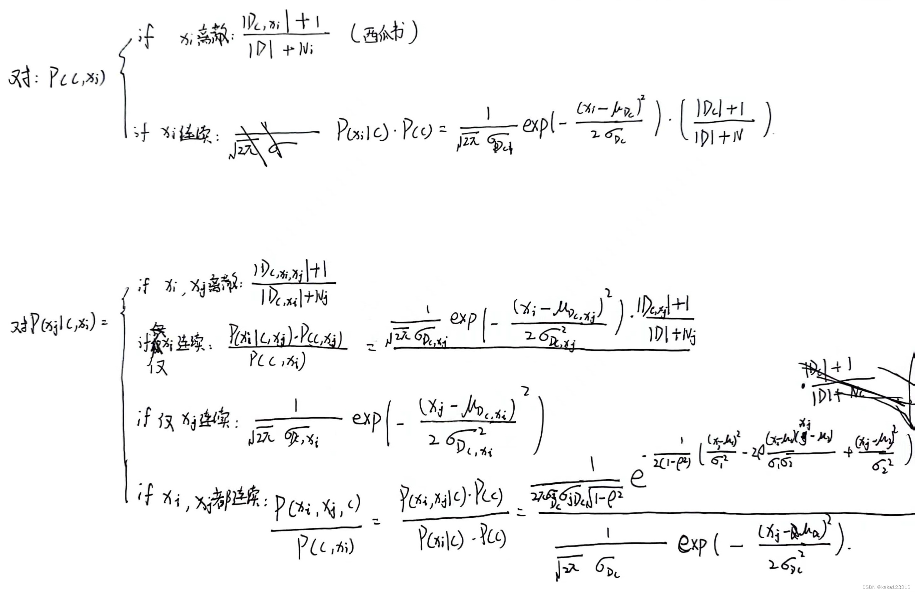
    def prior(self, ask_indexd, ask, c):#P（c|x）计算，此处传入的ask_indexd是单个数值，是向量化传入的，其余直接传入
        i_index = int(ask_indexd // 1000)#解码处
        l_index = int(ask_indexd % 1000)
        Di=self.data_extractor([i_index],l_index,ask,c='False')
        if Di.shape[0]<self.m:
            return 0
        if i_index in self.cvi:
            Dc = self.data_extractor([], l_index, ask, c)
            sigma1 = calculate_variance(Dc[:, i_index])
            u1 = calculate_mean(Dc[:, i_index])
            use1 = normal_distribution_probability(sigma1, ask[l_index, i_index], u1)
            use2 = (Dc.shape[0] + 1) / (self.z.shape[0] + self.category_quantity_query(-1))
            ret=use1 * use2
            return ret
        Dci = self.data_extractor([i_index], l_index, ask=ask, c=c)
        Ni = self.category_quantity_query(i_index)
        ret=(Dci.shape[0] + 1) / (self.z.shape[0] + Ni)
        return ret

    vprior = np.vectorize(prior, excluded=['ask'])

    def posterior(self, j_index, i_index, l_index, ask, c):#计算P（xj|c,xi）
        if j_index in self.cvi and i_index in self.cvi:
            data1 = self.data_extractor([], l_index, ask, c)
            sigma1 = calculate_variance(data1[:, i_index])
            sigma2 = calculate_variance(data1[:, j_index])
            p = calculate_correlation(data1[:, i_index], data1[:, j_index])
            u1 = calculate_mean(data1[:, i_index])
            u2 = calculate_mean(data1[:, j_index])
            use1 = joint_pdf(ask[l_index, i_index], ask[l_index, j_index], u1, u2, sigma1, sigma2, p)
            use2 = normal_distribution_probability(sigma1, ask[l_index, i_index], u1)
            return use2 / use1

        if i_index in self.cvi:
            Dcj = self.data_extractor([j_index], l_index, ask, c)
            if Dcj.size==0:
                return 0
            sigma1 = calculate_variance(Dcj[:, i_index])
            u1 = calculate_mean(Dcj[:, i_index])
            use1 = normal_distribution_probability(sigma1, ask[l_index, i_index], u1)
            Nj = self.category_quantity_query(j_index)
            use2 = (Dcj.shape[0] + 1) / (self.z.shape[0] + Nj)
            Dc = self.data_extractor([], l_index, ask, c)
            sigma2 = calculate_variance(Dc[:, i_index])
            u2 = calculate_mean(Dc[:, i_index])
            use3 = normal_distribution_probability(sigma2, ask[l_index, i_index], u2)
            use4 = (Dc.shape[0] + 1) / (self.z.shape[0] + self.category_quantity_query(-1))
            return (use1 * use2) / (use3 * use4)

        if j_index in self.cvi:
            Dci = self.data_extractor([i_index], l_index, ask, c)
            if Dci.size==0:
                return 0
            sigma1 = calculate_variance(Dci[:, j_index])
            u1 = calculate_mean(Dci[:, j_index])
            use1 = normal_distribution_probability(sigma1, ask[l_index, j_index], u1)
            return use1

        Dcij = self.data_extractor([i_index, j_index], l_index, ask, c)
        Dci = self.data_extractor([i_index], l_index, ask, c)
        Nj = self.category_quantity_query(j_index)
        return (Dcij.shape[0] + 1) / (Dci.shape[0] + Nj)

    vposterior = np.vectorize(posterior, excluded=['ask'])

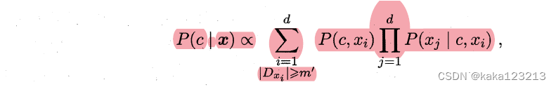
    def am_posterior(self, ask_indexd, ask, c):#计算累乘P（xj|c,xi）
        i_index = ask_indexd // 1000#解码处
        l_index = ask_indexd % 1000
        j_index = np.arange(0, ask.shape[1], 1)
        wait_to_mu = self.vposterior(self,j_index, i_index, l_index,ask=ask,c= c)
        ret=np.cumprod(wait_to_mu)[-1]
        return ret

    vam_posterior = np.vectorize(am_posterior, excluded=['ask','c'])

    def Judgment_function_by_c(self, ask, c):#计算P（c|x）
        ask_indexd = ask_index(ask)
        am = self.vam_posterior(self,ask_indexd=ask_indexd, ask=ask, c=c)
        pri = self.vprior(self,ask_indexd=ask_indexd, ask=ask, c=c)
        ret = np.multiply(am, pri)
        return np.sum(ret, axis=1)

    def pred(self, ask):#进行比较输出预测结果
        n = np.unique(self.z[:, -1])
        jude = np.array([])
        for c in n:
            judement = self.Judgment_function_by_c(ask, c)
            if jude.size==0:
                jude=np.expand_dims(judement,axis=1)
            else:
                jude=np.concatenate((jude,np.expand_dims(judement,axis=1)),axis=1)
        result=np.array([])
        for i in jude:
            result=np.append(result,n[np.argmax(i)])
        return np.expand_dims(result,axis=1)

if __name__ == '__main__':
    x, y = load_data()
    z = np.concatenate((x, y), axis=1)
    ask = x.astype(np.float32)
    mode = AODE_model(z, [6, 7],5)
    result=mode.pred(ask)
    print(result)

五、离散型数据处理思路：

        此代码对于离散型数据的处理，采用了正态分布函数进行处理：

附录：

一、数据集（来自西瓜书）：

二、计算公式