逻辑回归 breast-cancer 数据集处理

# -*- coding: utf-8 -*-

import pandas as pd
import numpy as np
from matplotlib import pyplot as plt
from sklearn.model_selection import train_test_split

def init():
    df = pd.read_csv("./breast-cancer.csv")
    
    # 处理无用列
    df = df.drop("id",1)
    df = df.drop("Unnamed: 32",1)
    
    # 处理标签列
    df['diagnosis'] = df['diagnosis'].map({
    	'M': 1,
    	'B': 0
    })
    
    # 划分训练集 (70%) 和测试集 (30%)
    train, test = train_test_split(df, test_size = 0.3, random_state=1)
    
    # 处理训练数据
    train_x = train.loc[:, 'radius_mean': 'fractal_dimension_worst']
    train_y = train.loc[:, ['diagnosis']]
    
    # 处理测试数据
    test_x = test.loc[:, 'radius_mean': 'fractal_dimension_worst']
    test_y = test.loc[:, ['diagnosis']]
    
    # 转换数据为np数组
    train_x = np.asarray(train_x)
    train_y = np.asarray(train_y)
    test_x = np.asarray(test_x)
    test_y = np.asarray(test_y)
    
    # 使用训练数据创建逻辑回归模型
    d = model(train_x.T, train_y.T, num_of_iterations=10000, alpha=0.000001)
    
    costs = d ["costs"]
    w = d["w"]
    b = d["b"]
    
    # 绘图
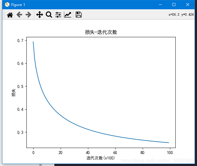
    plt.plot(costs)
    plt.title("损失-迭代次数")
    plt.xlabel("迭代次数(x100)")
    plt.ylabel("损失")
    
    # 计算精确度
    Y_prediction_train = predict(train_x.T, w, b)
    Y_prediction_test  = predict(test_x.T, w, b)
    
    print("\n训练数据测试精确度: {}%".format(100 - np.mean(np.abs(Y_prediction_train - train_y.T)) * 100))
    print("\n测试数据测试精确度: {}%".format(100 - np.mean(np.abs(Y_prediction_test - test_y.T)) * 100))
    
    plt.show()
    
    

# 初始化权值
def initialize(m):
    w = np.zeros((m,1))
    b = 0

    return w , b
    
# sigmoid函数    
def sigmoid(X):
    return 1/(1 + np.exp(- X))    

# 正反向传播
def propogate(X, Y, w, b):
    # 样本数量
    m = X.shape[1]

    # 正向传播 计算损失
    Z = np.dot(w.T, X) + b;    
    A = sigmoid(Z)
    cost= -(1/m) * np.sum(Y * np.log(A) + (1-Y) * np.log(1-A))
    
    # 反向传播 计算梯度
    dw = (1/m)* np.dot(X, (A-Y).T)
    db = (1/m)* np.sum(A-Y)
    
    grads= {"dw": dw, "db": db}
    return grads, cost


# 执行梯度下降
def optimize(X, Y, w, b, num_of_iterations, alpha):
    costs=[] 
    
    for i in range(num_of_iterations):
        grads, cost = propogate(X, Y, w, b)
        
        dw = grads["dw"]
        db = grads["db"]
        
        w = w - alpha * dw
        b = b - alpha * db
        
        # 每十次迭代存储一个损耗
        if i % 100 == 0:
            costs.append(cost)
            print("<%i>次迭代后的损失度: %f" % (i, cost))
            
    parameters = {
        "w": w, 
        "b": b
    }
    grads = {
        "dw": dw,
        "db": db
    }
    
    return parameters, grads, costs


# 对数据集进行预测
def predict(X, w, b):
    # 训练集数量
    m = X.shape[1] 
    
    y_prediction =  np.zeros((1,m))
    
    w = w.reshape(X.shape[0], 1)
    
    A=sigmoid(np.dot(w.T, X)+b)
    
    for i in range(A.shape[1]):
        if(A[0,i] < 0.5):
            y_prediction[0,i] = 0
        else:
            y_prediction[0,i] = 1
    
    return y_prediction


# 计算逻辑回归模型
def model(Xtrain, Ytrain, num_of_iterations, alpha):
    # 获取特征数量
    dim = Xtrain.shape[0] 
    
    w,b = initialize(dim)
    
    parameters, grads, costs = optimize(Xtrain, Ytrain, w, b, num_of_iterations, alpha) 
    
    w = parameters["w"]
    b = parameters["b"]
    
    d = {
        "w": w,
        "b": b, 
        "costs": costs
    }
    
    return d
    
if __name__ == "__main__":
    init()